Home Project 1 Project 2 Project 3 Project 4 Project 5

Fun With Diffusion Models!

Part A: The Power of Diffusion Models!

Introduction

Recently, diffusion models have been demonstrated to achieve better image generation than GANs, while also having a much more stable training regime that avoids the instability and mode collapse associated with adversarial learning. Diffusion models accomplish this by learns to gradually denoise an image, a process that can be learned through simple supervised learning predicting the noise of an image gradually being made more noisy, and then using DDPM sampling to "play the tape in reverse" to create images from noise. In this part, we will use a pretrained diffusion model DeepFloyd IF, and explore how to use this model to implement DDPM sampling, image to image transformations, and more.

Part 0: Setup

To first use the model, we needed to download the model from HuggingFace. After setting up the model, we generate some outputs from the model, varying the number of inference steps. The outputs are shown below:
Prompt 10 Inference Steps 20 Inference Steps
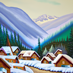
an oil painting of a snowy mountain village 10 Inference Steps 20 Inference Steps
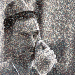
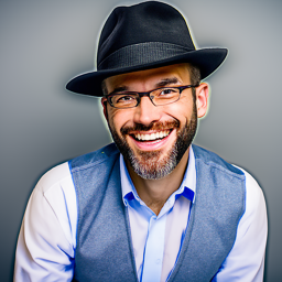
a man wearing a hat 10 Inference Steps 20 Inference Steps
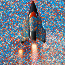
a rocket ship 10 Inference Steps 20 Inference Steps
We can see that the outputs generated with 20 inference steps are much clearer and better, which shows how more sampling steps can increase output quality. The outputs seem to match the text prompts quite well. My random seed is 180.

Part 1: Sampling Loops

1.1: Forward Process
In this part, we implement the forward process of adding Gaussian noise to an input image to sample from the distribution at any timestep conditioned on the original input. This is equivalent to scaling the input by the square root of alpha_hat at timestep t, and adding Gaussian noise scaled by the square root of 1 - alpha_hat at timestep t. We visualize the result at t=0, 250, 500, and 750 below:
t = 0 t = 250 t = 500 t = 750
Part 1.2: Classical Denoising
We can attempt to remove the noise by doing classical denoising; applying a Gaussian blur to remove the noise. This does not work well because we cannot recover the high frequency information that has been lost. The results of this are shown below.
t = 250 t = 500 t = 750
Noisy Image t = 250 t = 500 t = 750
Denoised Image t = 250 Denoised t = 500 Denoised t = 750 Denoised
Part 1.3: One-Step Denoising
We can also use the learned diffusion model to try to remove all of the noise in a single step. The original image is the same as above. We show the results of this single-step denoising and the original image. We note that while it is much better than classical methods, it still struggles to fully reproduce the original image.
Original Image
t = 0
t = 250 t = 500 t = 750
Noisy Image t = 250 t = 500 t = 750
Denoised Image t = 250 Denoised t = 500 Denoised t = 750 Denoised
Part 1.4: Iterative Denoising
We note that it gets worse as there is more noise to remove, which makes sense, as it is quite difficult to accurately project back to the image all at once. We use DDPM to implement iterative denoising, and visualize the results below. We see that it performs much better. We give the input a noisy image that corresponds to t=690, and perform iterative denoising from there. We compare it to the one-step denoising and Gaussian blur denoising.
Noisy Campanile at t = 90 Noisy Campanile at t = 240 Noisy Campanile at t = 390 Noisy Campanile at t = 540 Noisy Campanile at t = 690
t = 90 t = 240 t = 390 t = 540 t = 690
Original Iteratively Denoised Campanile One-Step Denoised Campanile Gaussian Blurred Campanile
Original Image Iteratively Denoised One-Step Denoised Gaussian Blurred
Part 1.5: Diffusion Model Sampling
We can use this same procedure to sample unconditional images from the model by providing pure noise as the original input. We visualize five generated images below:
Sample 1 Sample 2 Sample 3 Sample 4 Sample 5
Part 1.6 Classifier-Free Guidance
We see that these outputs are not very good, so we can try to use classifier-free guidance, where a model is trained on both paired conditional generation and unconditional generation. Then, at sampling time, we extrapolate the noise predicted for the conditional generation away from the unconditional generation. We use a CFG scale parameter of 7, and the prompt "a high quality photo" for conditional generation. We visualize five samples from this process below:
Sample 1 Sample 2 Sample 3 Sample 4 Sample 5
Part 1.7 Image-to-image Translation
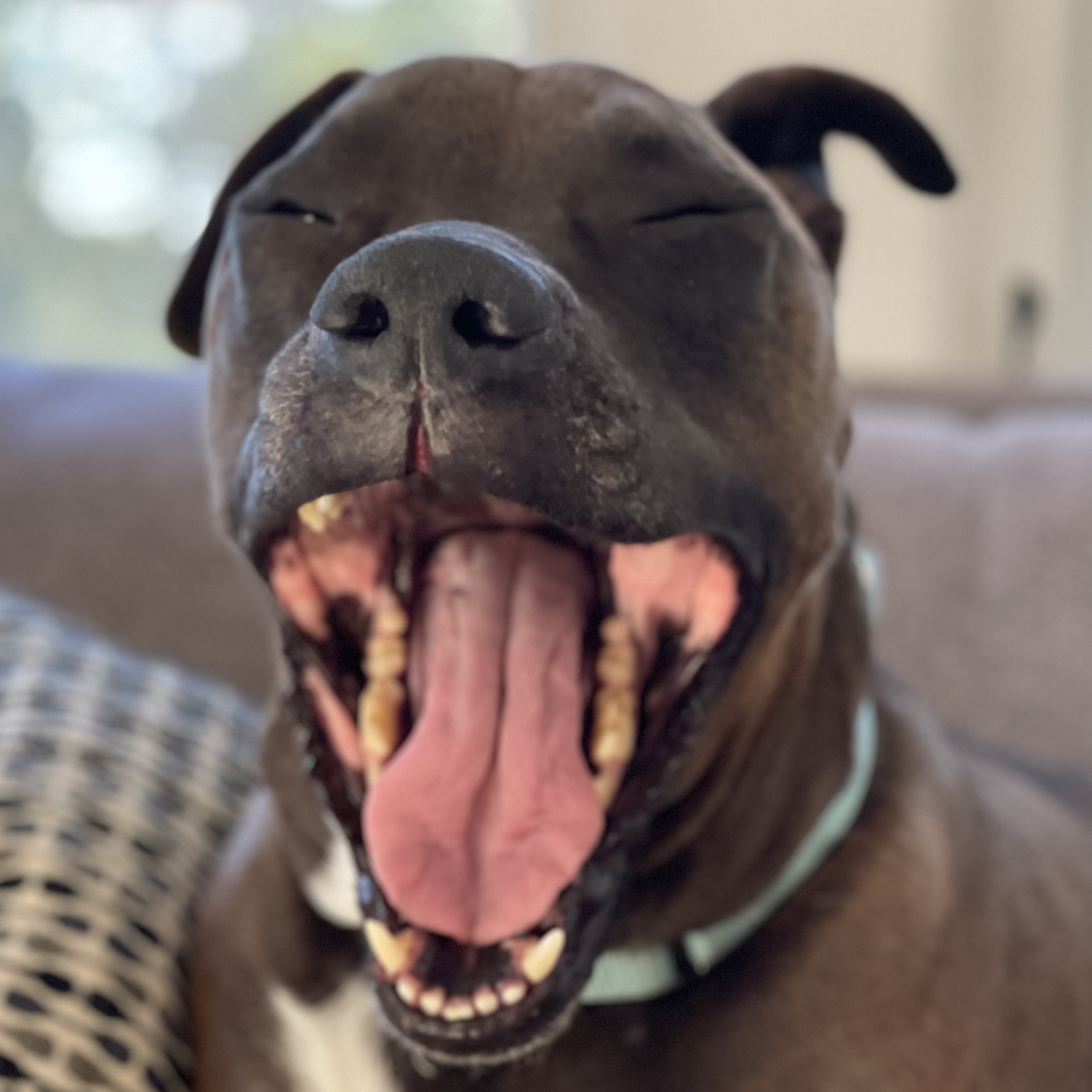
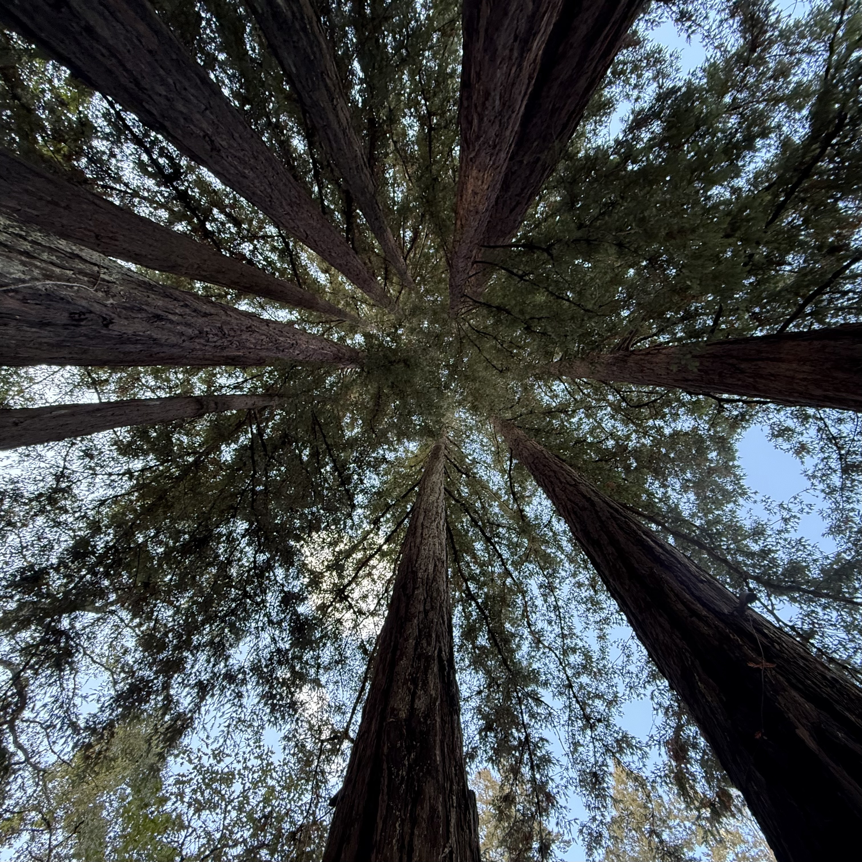
We see that we can get edits of images by giving the model a noised version of that image, and seeing how it projects the image back onto the manifold. We do this for three images, and observe that the image gradually looks more and more like the original image. The two images other than the Campanile were taken by me.
SDEdit with i_start=1 SDEdit with i_start=3 SDEdit with i_start=5 SDEdit with i_start=7 SDEdit with i_start=10 SDEdit with i_start=20 Original Image
campanille i_start=1 campanille i_start=3 campanille i_start=5 campanille i_start=7 campanille i_start=10 campanille i_start=20 Original Image
bear i_start=1 bear i_start=3 bear i_start=5 bear i_start=7 bear i_start=10 bear i_start=20 Original Image
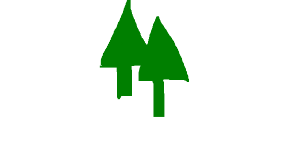
trees i_start=1 trees i_start=3 trees i_start=5 trees i_start=7 trees i_start=10 trees i_start=20 Original Image
Part 1.7.1 Editing Hand Drawn Images and Web Images
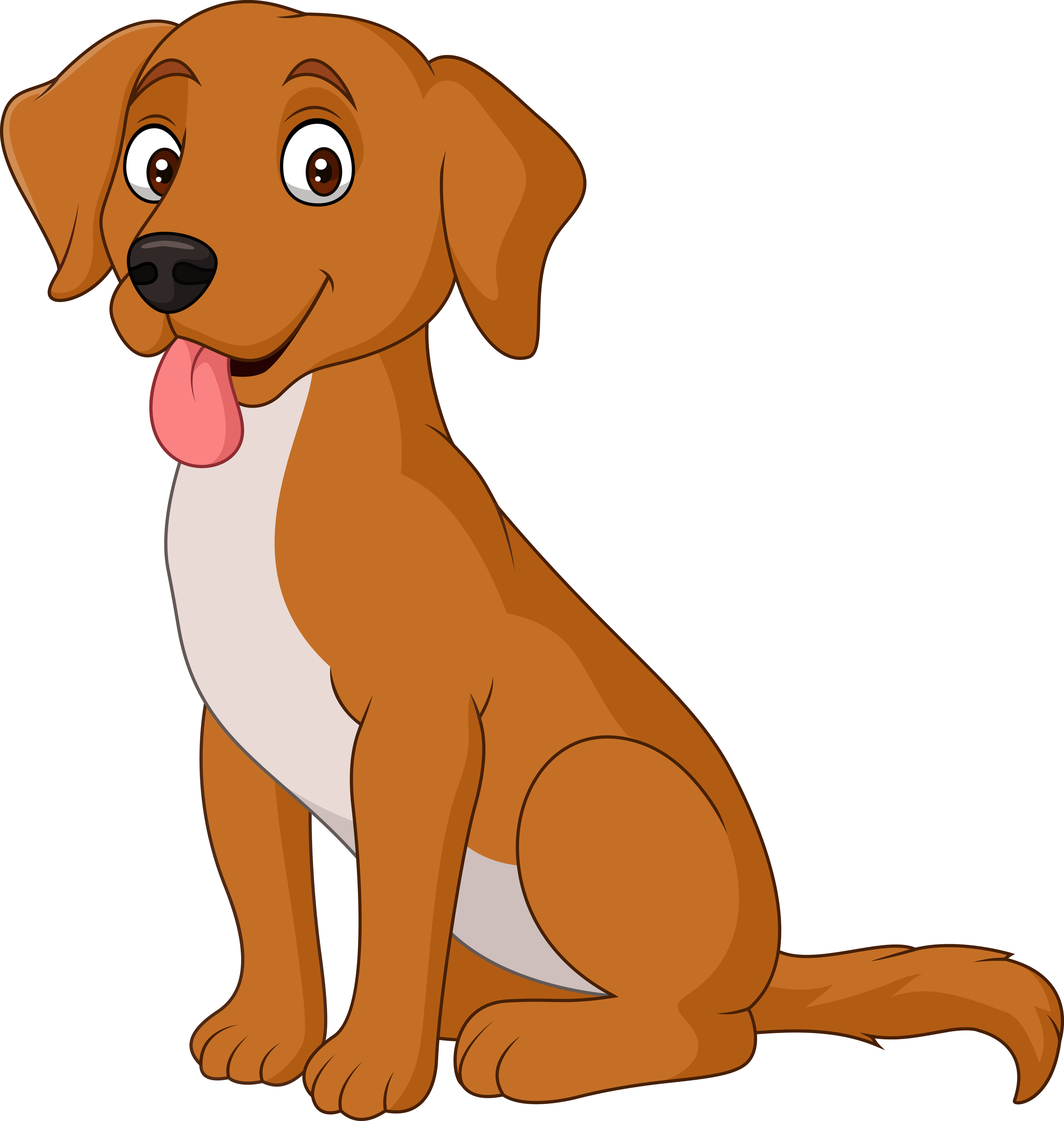
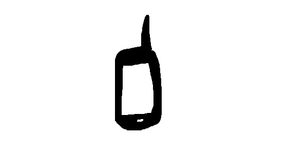
We can apply the same method to images that are sketches, and see the model interpolate details and make things look more photorealistic. The two sketches were done by me, the cartoon dog is from Adobe Stock.
SDEdit with i_start=1 SDEdit with i_start=3 SDEdit with i_start=5 SDEdit with i_start=7 SDEdit with i_start=10 SDEdit with i_start=20 Original Image
campanille i_start=1 campanille i_start=3 campanille i_start=5 campanille i_start=7 campanille i_start=10 campanille i_start=20 Original Image
bear i_start=1 bear i_start=3 bear i_start=5 bear i_start=7 bear i_start=10 bear i_start=20 Original Image
trees i_start=1 trees i_start=3 trees i_start=5 trees i_start=7 trees i_start=10 trees i_start=20 Original Image
1.7.2 Inpainting
We can also use the same procedure as above, but instead mask part of the image and have the model interpolate what was there before. We force the image to match the noised version of the original image at each step for parts of the image that are masked. In can take multiple attempts, since this is not specifically what the model was trained to do. We visualize the results of this on three images: the Campanile, a photo of a Shiba Inu (Adobe Stock), and a MacBook Pro (Adobe Stock). We see that the model correctly interpolates a reasonable top of the Campanile, as well as adds eyes back to the Shiba Inu. In removes the logo from the MacBook Pro in most runs, though there was one run (unfortunately not saved) where it did start to reconstruct something resembling an Apple logo.
Original Image Mask Reconstructed Image
campanille original campanille mask campanille reconstructed
shiba inu original shiba inu mask shiba inu reconstructed
None original None mask None reconstructed
Part 1.7.3 Text Conditional Image-to-image Translation
We note that we can also do image-to-image translation with a prompt for guidance. We do the same images as in 1.7.0, but add the prompts as show in the table below:
Prompt SDEdit with i_start=1 SDEdit with i_start=3 SDEdit with i_start=5 SDEdit with i_start=7 SDEdit with i_start=10 SDEdit with i_start=20 Original Image
a rocket ship campanille i_start=1 campanille i_start=3 campanille i_start=5 campanille i_start=7 campanille i_start=10 campanille i_start=20 Original Image
a photo of a dog dog i_start=1 dog i_start=3 dog i_start=5 dog i_start=7 dog i_start=10 dog i_start=20 Original Image
a photo of the amalfi coast trees i_start=1 trees i_start=3 trees i_start=5 trees i_start=7 trees i_start=10 trees i_start=20 Original Image
Part 1.8: Visual Anagrams
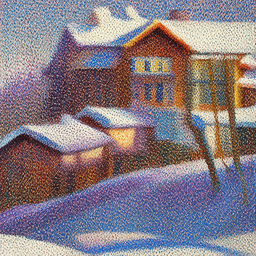
We note that we can also create visual anagrams by elegantly combining the noise estimates for two different prompts. We feed two prompts, one for what the image should look like right-side up and the other for what it should look like upside down. Then, at each step, we get the predicted noise from the model for the image right-side up under guidance of right-side up prompt, and the predicted noise for the image upside down for the upside down prompt. Then, we average the right side up noise estimate with the vertically flipped noise estimate for the upside down prompt. Empirically, I found that placing more weight on the prompt with less signal led to better results. The weight listed below is the weight for the right-side up prompt. Below, I visualize the results for three visual anagrams.
Prompt Flipped Prompt Weight Image Flipped Image
an oil painting of people around a campfire an oil painting of an old man 0.75 oil painting campfire flipped oil painting campfire
a photo of a hipster barista an oil painting of a snowy mountain village 0.65 hipster barista flipped hipster barista
a lithograph of waterfalls a lithograph of a skull 0.75 waterfalls lithograph flipped waterfalls lithograph
Part 1.9: Hybrid Images
We can apply a very similar technique to get hybrid images, which look like one thing close up and another thing far away. This is the same as in project 2, where we want the low frequency components of one image and the high frequency components of another. We can achieve this by getting the predicted noise for each image, and then adding a low-pass filtered version of the low-pass image noise prediction to the high-pass filtered version of the high-pass image noise prediction. We visualize the results for three hybrid images below.
Low Freq. Prompt High Freq. Prompt Image
a lithograph of a skull a lithograph of waterfalls waterfall and skull lithograph
a lithograph of a cat a lithograph of a dog dog and cat lithograph
a lithograph of a man a lithograph of a skull skull and man lithograph
We note that for the last two, the output is largely the body of the low frequency prompt and the head of the high frequency prompt. This makes sense, since from far away it is difficult to make out the details of the face, so you assume the whole thing is likely the identity of the body (in this case, cat for the second and man for the third). But as you get closer, you see the details in the face, which reveals the high frequency prompt.

Part B: Diffusion Models from Scratch!

Introduction

Now, we can try to train a small diffusion model from scratch to generate digits based on the MNIST digit dataset. This involves creating a model, training the model, and implementing the sampling loop. We additionally use classifier-free guidance to generate specific digits.

Part 1: Training a Single-Step Denoising U-Net

1.1 Implementing the U-Net

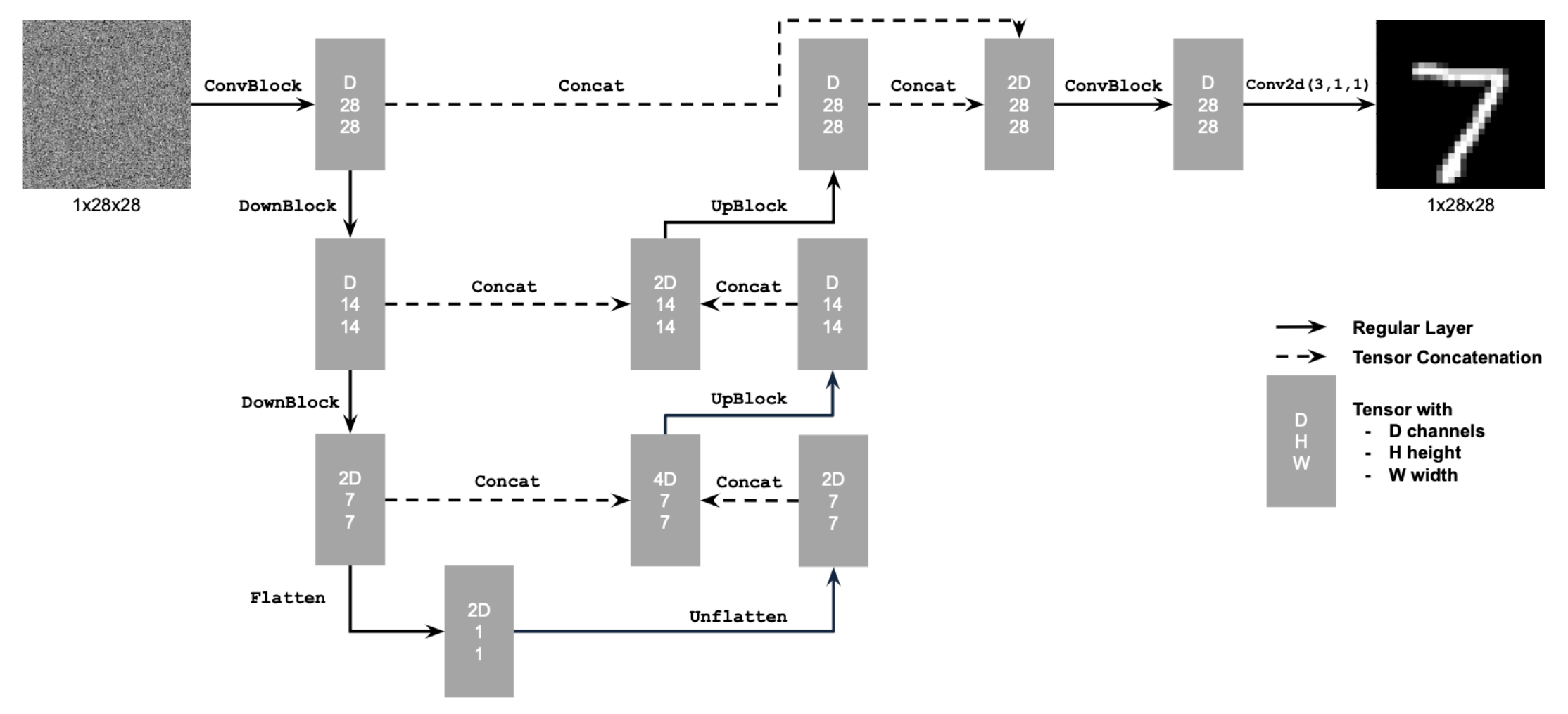
For our model architecture, we use a UNet, which assures that the information and different levels is appropriately propagated to later layers by having skip connections. The image is repeatedly downsampled to learn a good representation, and then upsampled, concatenating with the corresponding downsampled image, to assure that no information is loss.
UNet Model Architecture
UNet Model Architecture (from project spec)

1.2 Using the UNet to Train a Denoiser

1.2.1 Training

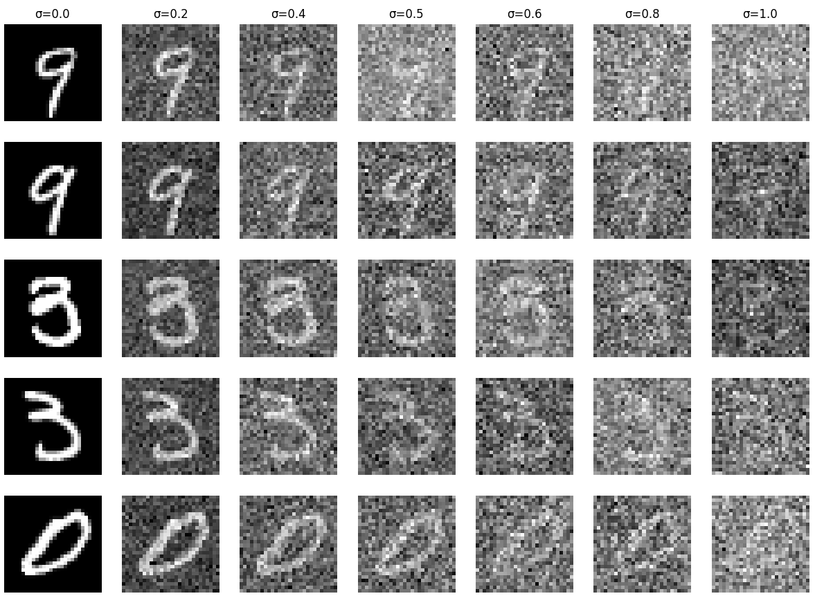
We use the UNet to learn a model to predict the noise added to the image during the forward process. We train the model to minimize the L2 loss with the true noise. To generate training samples, we sample original images, and add noise to them. In the figure below, we visualize what different datapoints from MNIST look like after adding different amounts of noise:
UNet Model Architecture
Varying levels of noise on MNIST digits
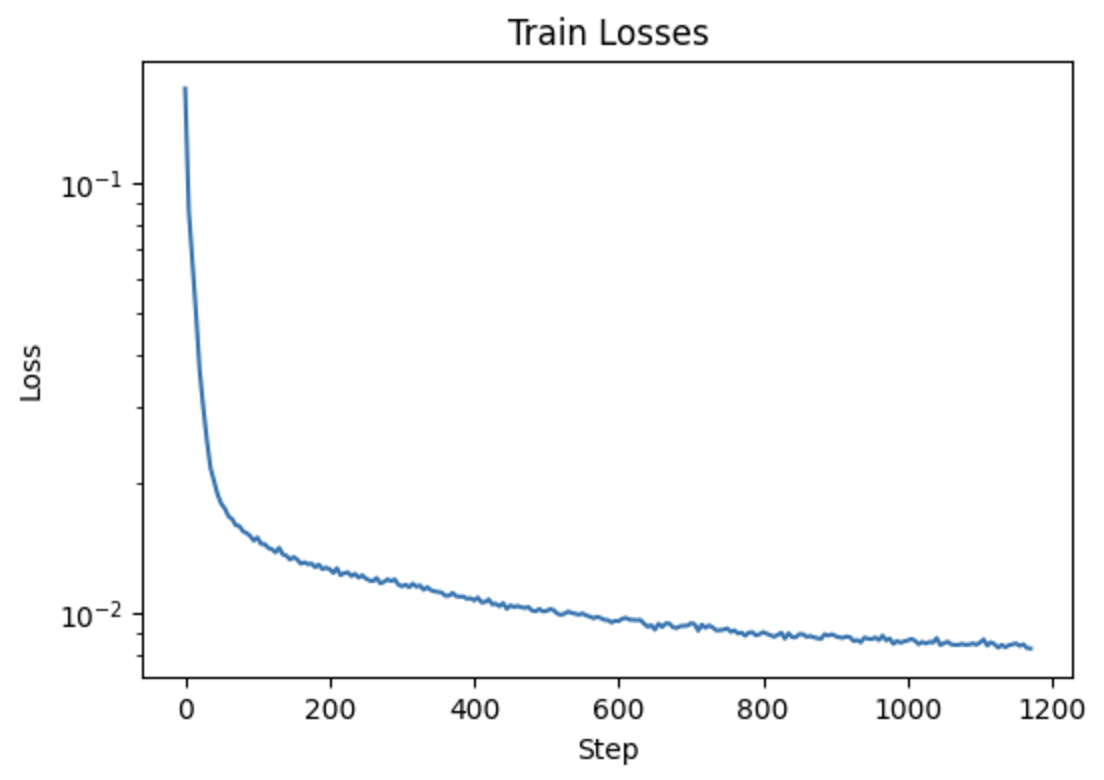
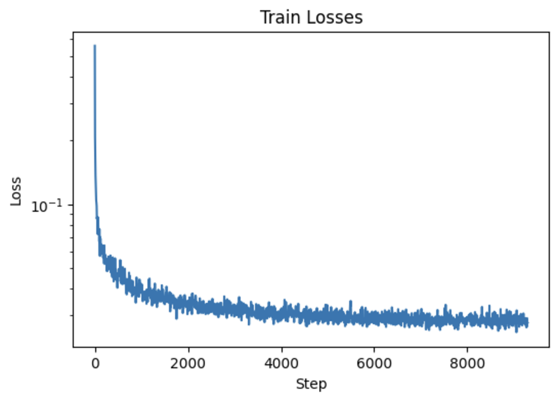
We can train the UNet using MSE loss to predict the noise added to the image. Since we are doing one step prediction, we will fix the noise quantity to have sigma = 0.5. We train for 5 epochs, batch size 256, learning rate 1e-4 using Adam, and a hidden dimension D of 128. We show the training loss below (averaging every 5 batches):
UNet Model Architecture
Training Loss Curve
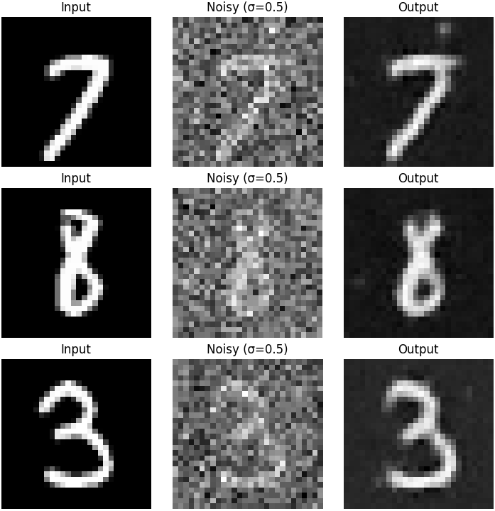
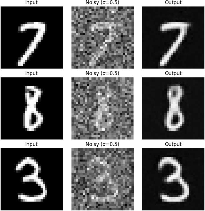
We now test the model by visualizing results after the 1st and 5th epoch:
UNet Model Architecture
Results on digits from the test set after 1 epoch of training
UNet Model Architecture
Results on digits from the test set after 5 epoch of training

1.2.2 Out-of-distribution Testing

We can also test how well the model generalizes to reconstructing images with more or less noise than it was trained on. We see that it generalizes well to less noise, but struggles when there is more noise. This suggests that using an iterative approach may work better for reconstructing images from pure noise.
UNet Model Architecture
Results on digits from the test set with varying noise levels.

Part 2: Training a Diffusion Model

2.1 Adding Time Conditioning to U-Net

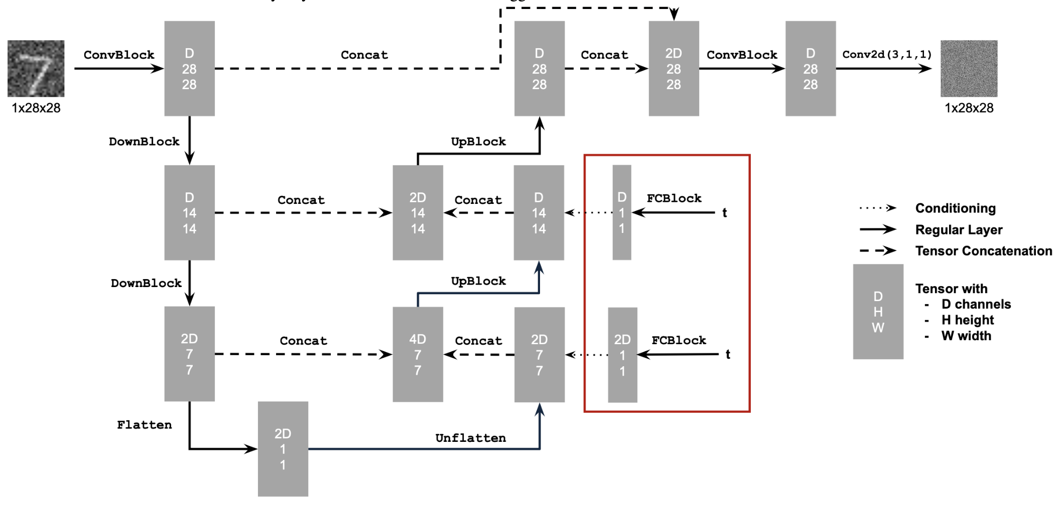
In order to perform DDPM sampling like we did in Part A, we need to train a UNet that predicts noise that is conditioned on the time (since the noise schedule changes over time). It has also been shown that conditioning on time makes the process more stable. To do this, we add two fully connected blocks to encode the time, and concatenate the time embedding to the input to each upsampling block of the UNet. The diagram below shows the details of the architecture:
UNet Model Architecture
Time-Conditioned UNet Model Architecture (from project spec)

2.2: Training the UNet

We train our UNet, selecting a random timestep for each element of the batch, computing the noisy image using the forward process, and then regressing the output of the network to the true noise. We train for 20 epochs, with batch size of 128, hidden dimension of 64, learning rate of 1e-3 with Adam optimizer, and exponential decay learning rate schedule with gamma = 0.01^(1/20). We show the training loss below (averaging every 5 batches):
UNet Model Architecture
Time-Conditioned UNet training loss curve

2.3: Sampling from the UNet

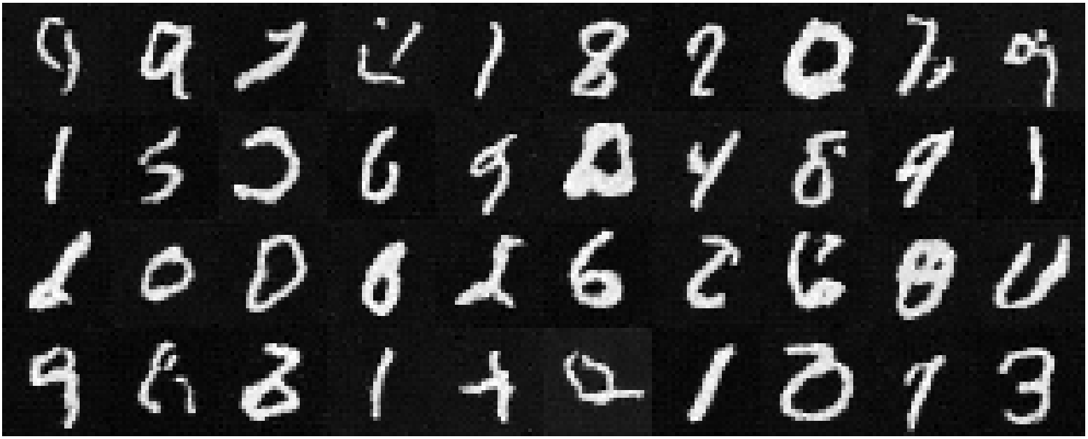
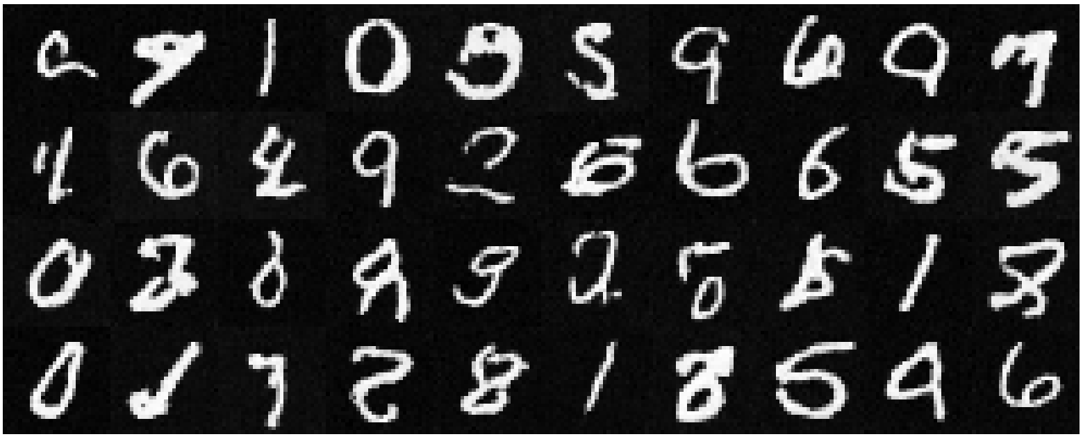
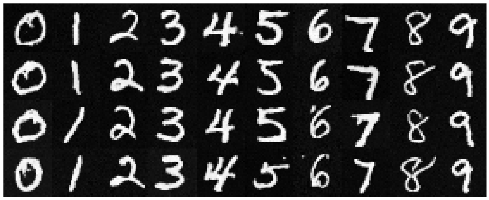
We implement DDPM sampling, and show the examples of sampled images from the model after 5 and 20 epochs of training.
UNet Model Architecture
Sampling results 5 epochs of training
UNet Model Architecture
Sampling results after 20 epochs of training
We see that while the quality is reasonable, some digits don't look that accurate, and it is not possible to sample specific digits. To fix this, we will implement classifier-free guidance.

2.4: Adding Class-Conditioning to UNet

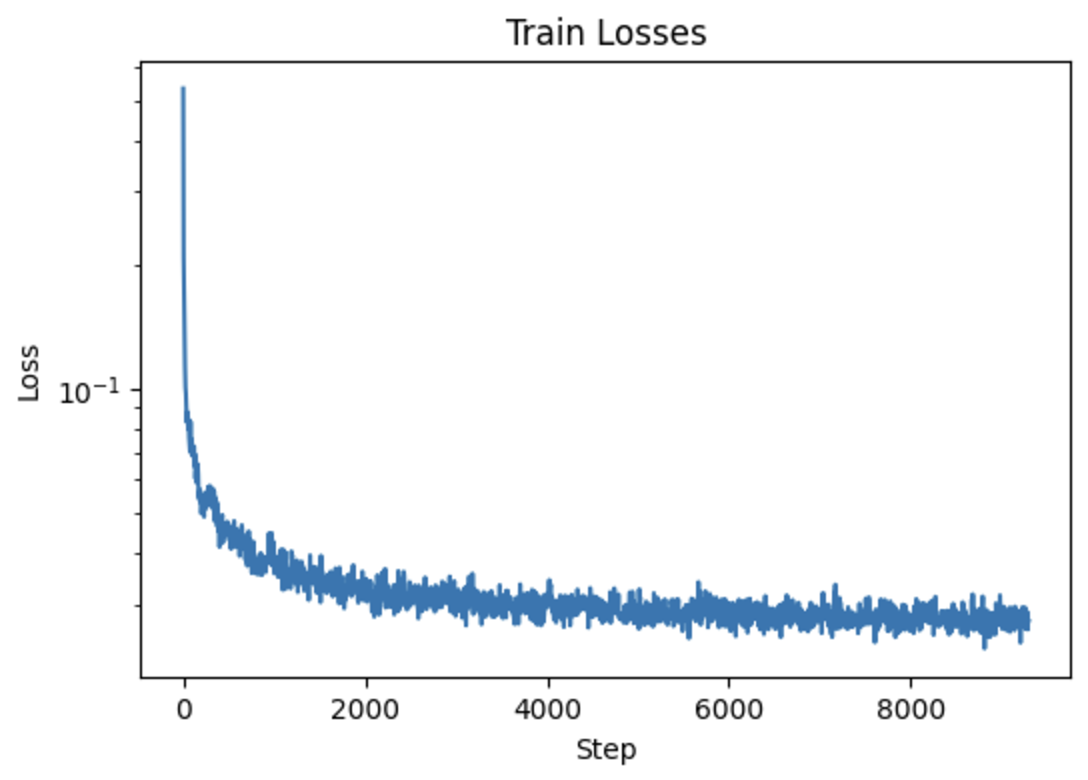
To add class conditioning, we encode the digit as a one-hot vector, and pass it into a similar fully connected block as the time in the previous section. We add the class embedding to the input of the UNet at each upsampling block, like we did for the time embedding. We drop the label with probability 0.1 to make sure the model learns unconditional generation as well. Then, as we did in part A, we implement classifier-free guidance sampling from the network. The training loss is shown below:
UNet Model Architecture
Class-Conditioned UNet training loss curve

2.5 Sampling from the Class-Conditioned UNet

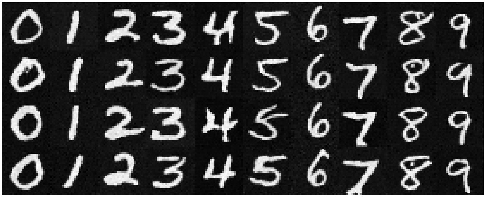
We show the results of sampling with classifier-free guidance after 5 and 20 epochs of training below, using a guidance scale of 5:
UNet Model Architecture
Sampling results 5 epochs of training
UNet Model Architecture
Sampling results after 20 epochs of training