Home Project 1 Project 2 Project 3 Project 4 Project 5

Face Morphing

Introduction

In this project, we explore face morphing. We create smooth morphs between different faces, analyze and create averages of many faces, and look at how population means can be used to caricatures. At a high level, this project morphs faces by first manually selecting many correspondence points on each face, then computing the average location of these points (aka, the average shape). Next, a triangulation is created that minimizes the angles within each triangle (to avoid being close to degenerate triangles). We we use the Delaunay triangulation method, which efficiently computes the triangulation with the smallest angles in O(n log n) time. We then compute the transformation for each triangle in the original images to same triangle in the current morph frame (weighted average of two point positions). Because it avoids "holes" where the current pixel in the original image maps to a location in between pixels in the destination, we invert the transformation and instead fill positions in the destination by interpolating from pixels in the original image. Finally, once both pictures are morphed to the same shape, we linearly mix the colors. Doing this for many frames with different shape/color linear ratios (I use linear for both) leads to a morph sequence. We extend this to look at face datasets, where we morph all images to the average face shape and compute the average color of morphed faces to get an average in the population. I then explore morphing my face on the average and vice versa, and creating caricatures by extrapolating from the mean. For the B & W, I also look at doing morphing and caricatures in the PCA basis.

Part 1: Defining Correspondences

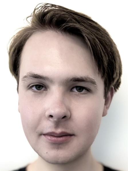
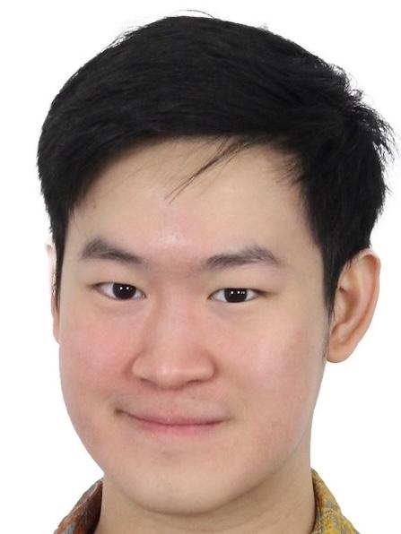
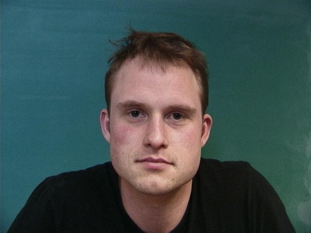
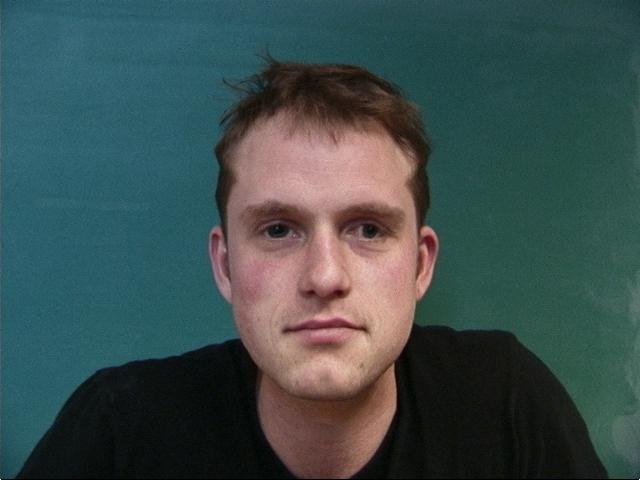
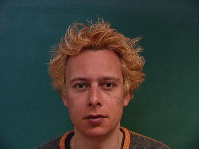
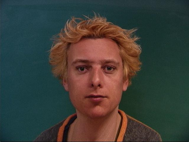
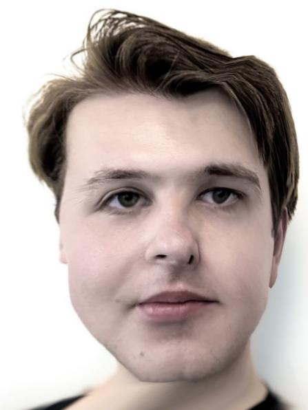
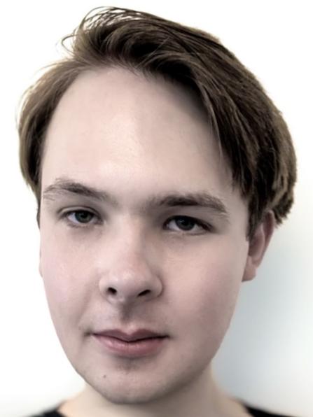
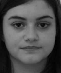
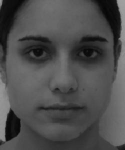
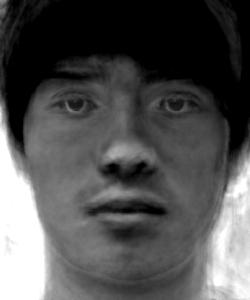
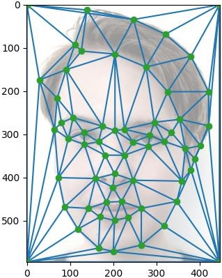
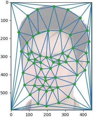
First, we need to find correspondences between our two images. My two images are me and my friend (also in CS 180) Brayton. I use this tool to compute correspondences. I average the points, and use scipy.spatial.Delaunay to compute the triangulation. I average the points first since I want the triangulation to be good for as much of the morph as possible. Below are my two images, with the correspondences and triangulation superimposed above the image:
Me (Max) Brayton

Part 2: Computing the Mid-Way face

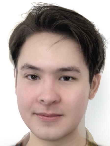
To compute the mid-way face, we take the average shape (average all correspondence points), and warp each triangle of each original image to that midway shape, and then average the color values. As described above, for warping the images, it is better to find the inverse transformation (mid-way shape to each original image) and interpolate the value of a pixel in the midway shape based on the pixels surrounding the corresponding location in the original image. For efficiency, I compute all of the transformed points first, and only make one call to scipy.interpolate.griddata. An earlier implementation made a call to scipy.interpolate.griddata for each triangle. Interestingly, this was very important for runtime, which suggests that there is a lot of overhead with making each call. Below are the two original images and mid-way face:
Me (Max) Brayton
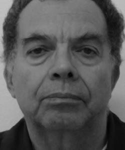
Camerman
Mid-way Face

Part 3: The Morph Sequence

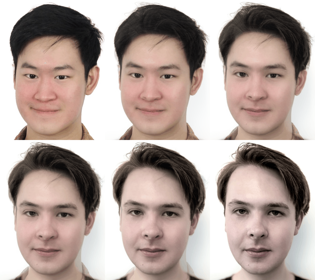
We do the same as above, but generalize the process to have a parameter to control the shape as a weighted average of the correspondences for each image, and the color to be a weighted average of each original image warped to the shared shape. I generated a 45 frame morph sequence, and found that a linear schedule for both the shape warp and color mix worked quite well. Below is the morph sequence of the above images:
Morph Sequence Brayton Max
Morph Sequence: Brayton to Me

Part 4: Computing the Average Face

To compute the average face, we use a dataset of faces with annotated correspondences, and use the morph approach above to morph each image to the average shape, and then average the pixel values. To accelerate the runtime for this process, I implemented multi-core parallelism using the multiprocess library to fully use all 12 cores on my laptop. To use the labelled datapoints in the dataset, I needed to extract the text values from the given text files, and preprocess them accordingly to be in pixel coordinates. I also added extra points in the corners, so the average image can use the whole image. Here are some examples from the Danish dataset of individual faces warped to the average shape:
Original Image Warped Image

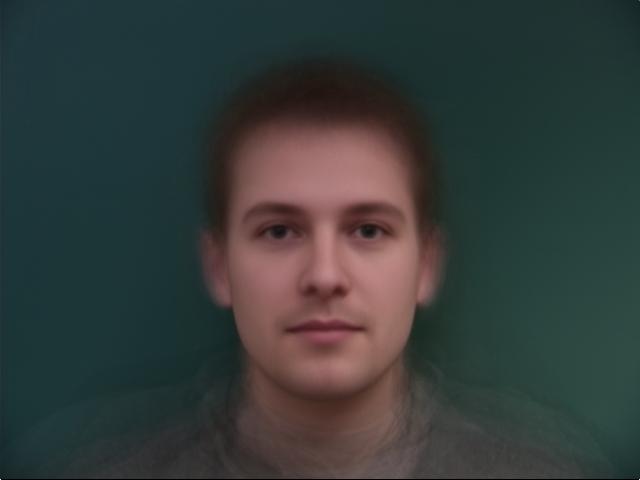
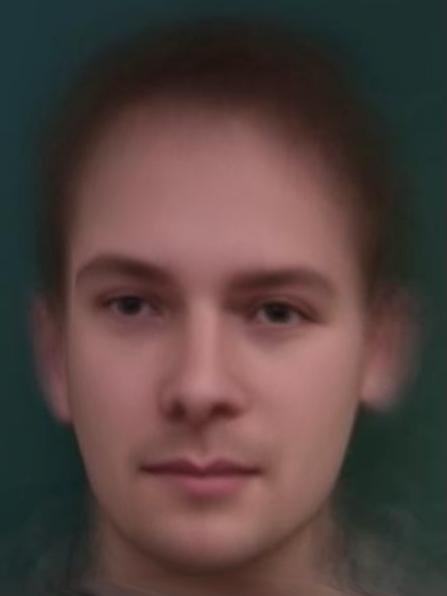
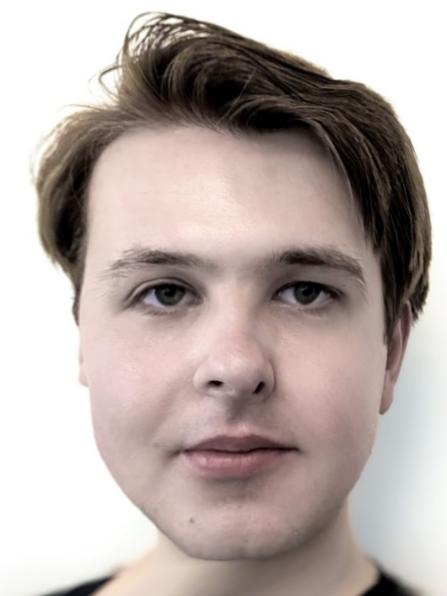
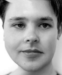
Below is the average face, average face morphed to my shape, and me morphed to average face shape for the Danish dataset.
Camerman
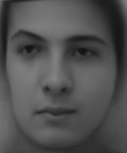
Average Face (Danish Dataset)
Average Face to My Geometry My Face to Average Face Geometry
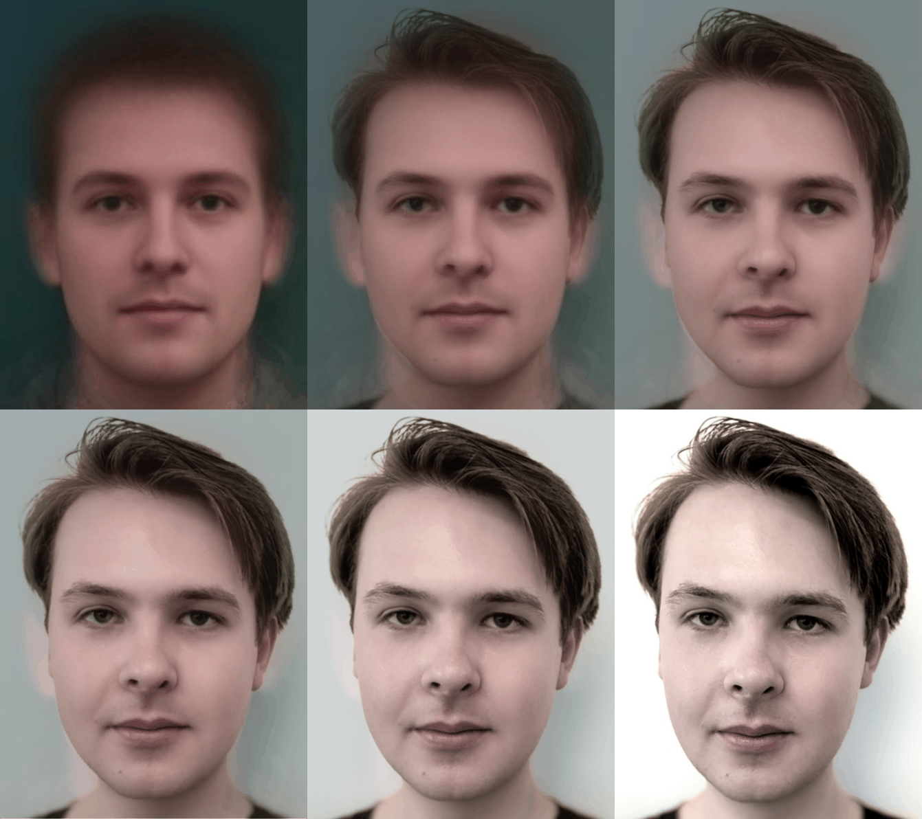
We can see that some aspects of the general differences in face shape are reflected here, for example it seems that my face is a bit more narrow than the average Danish face. However, we also see that the alignment of the original images is very important. My head is turned ever so slightly to the right, so the space on the left side of the image is smaller on my face image vs the average person from the Danish set. This leads to a compression of the average face warped to my geometry, and a stretching on my face to the average geometry. I also did not match any keypoints for the ears or outer hairline, since these features are quite blurry in the average. I also include a morphing of the average Danish face to me:
Morph Sequence Brayton Max
Morph of Average from Danish Dataset to Me
I also compute the same results for the FEI dataset:
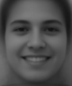
Average Face, FEI, Neutral Average Face, FEI, Smiling
Average Face to My Geometry My Face to Average Face Geometry
Morph Sequence Brayton Max
Morph of Average from FEI Dataset to Me

Part 5: Extrapolating From the Mean

To create a caricature of myself by extracting from the mean, I perform the same interpolation as I used for making the morph sequence, except in this case my two images are me and the average from the previous step (in this case, averages from Danish dataset and FEI dataset). To make this extrapolation, I use alpha values of -0.5 and 1.5 for the shape morph. Higher alpha accentuates my features with respect to the average more. Below are the caricatures of me from the mean of the two different datasets:
Danish Dataset, Alpha = -0.5 Danish Dataset, Alpha = 1.5
FEI Dataset (Neutral), Alpha = -0.5 FEI Dataset (Neutral), Alpha = 1.5
Similar to the results in the previous section, we see that the most obvious accentuated change is making the left side of my face wider/narrower, because my picture is not quite at a head on angle, so the left side of my face is slightly more narrow.

Bells + Whistles: Caricatures and Transformations in PCA Basis

Principle component analysis is a mathematical way of computing the vectors that point in the directions that have the most variance in the underlying data. The EigenFaces project showed that faces can be approximated with relatively few principle components, keeping important information while ignoring noise. This leads to the thought that doing these facial morphs and transformations in a PCA basis may lead to interesting results.

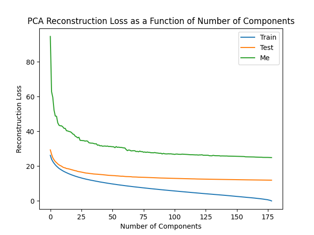
I compute the PCA basis for unmodified images from the FEI dataset used above, as there were more images, so I felt that the features might generalize better. To test how much the vectors were fit to the specific training corpus, I did a randomized 90-10 train-test split. Since I also wanted to use this basis to create a caricature of myself, I decided to plot the reconstruction loss as a function of number of PCA components for training set, test set (still from FEI dataset), and me. The loss plot is shown below:
Morph Sequence Brayton Max
PCA Loss as a function of number of components.
From this plot, we see that around 30 principle components, the test loss decreases quite slowly, but the train loss continues to decrease towards 0 (since at the full number of components, its just a change of basis with no loss in expressiveness). We want to use enough components to be able to represent the images, but not so many components that we don't throw any information away, since then it reduces to linearly combining the original images. We also see that any number of PCA components struggles to reproduce my original image after projection. This suggests that my face does not match the training distribution.

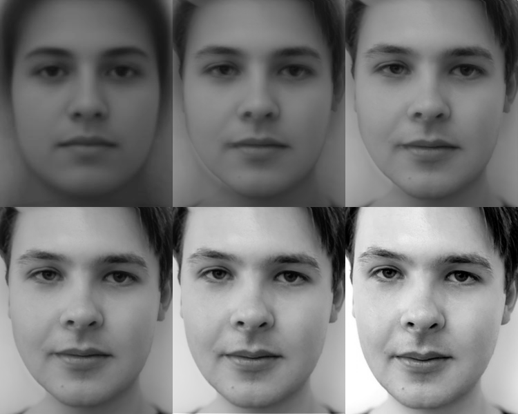
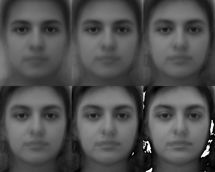
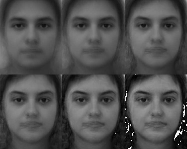
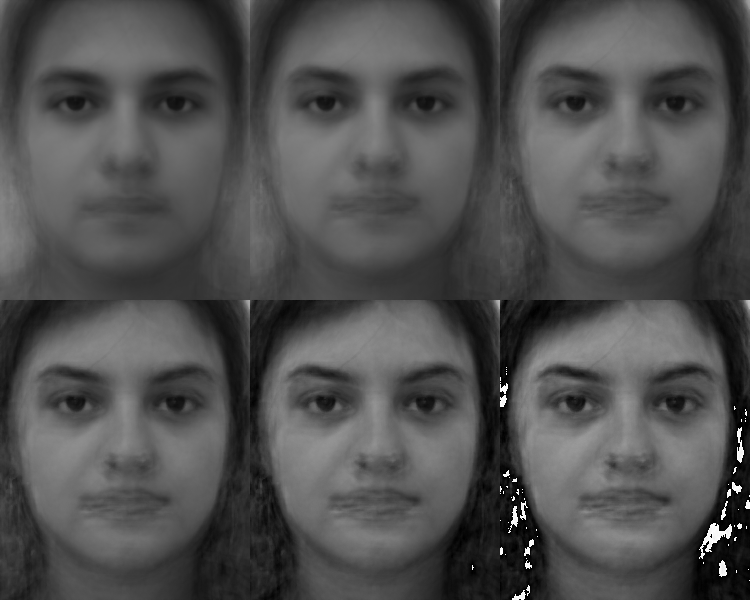
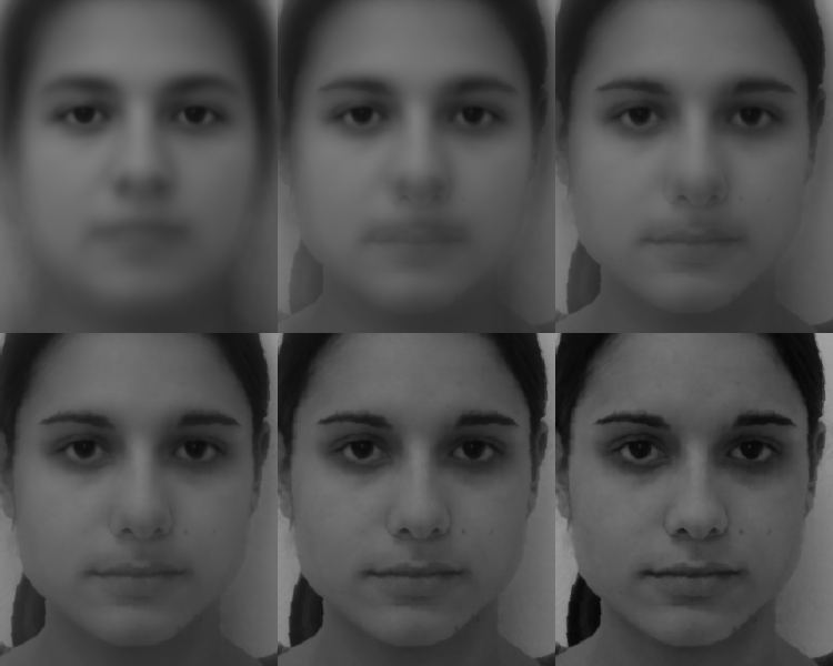
Below, I show a few different morphs in this basis. To perform the morph, I project each image into the PCA space, linearly interpolate within the PCA basis, and then project back in the normal space. First, I show the final images of the morph. Then, I show morphs with 30, 120, and 180 (full cross dissolve for train set) principle components.
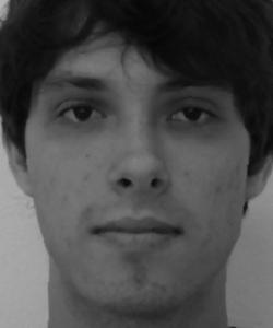
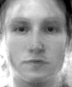
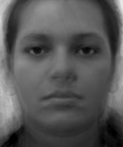
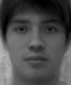
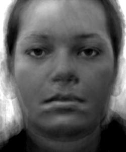
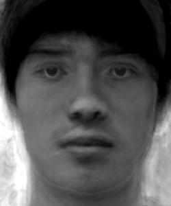
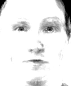
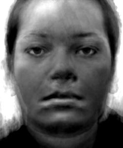
Average of Train Images to Me Average of Test Images to Random Test Image Average of Train Images to Random Train Image
We see that all of these morphs look a bit like a simple cross dissolve, which makes sense since the PCA basis is linear. However, I think it is not quite as obvious when there are fewer numbers of principle components (ie. 30). It is also much faster since there are no shape transformations. However, the trade off is a blurrier image and poor generalization if the image is quite different than the dataset. As a result of this, we see fringing/clipping for the test image and me as the number of components increases.

Next, we look at using this PCA based approach for caricatures. To do this, we perform interpolation in the PCA basis as above but take an alpha that is larger than 1 to accentuate differences between the target image and the average. For me and a random train image I use the train average to start, for the test image we extrapolate from the test average. We use 30 principle components.
Me From Train Average Test Example from Test Average Train Example From Train Average
Target Image
Target Image PCA
Reconstruction
Alpha = 1.5
Alpha = 2
Alpha = 3
We see that this effectively just increases the contrast, since we have removed some of the "noise" by projecting to a lower dimensional space, and then are linearly extrapolating in this space. Thus, it makes sense that we would mostly see an accentuation of brightness intensity differences. Additionally, we see that the test image and me are not as well reproduced, leading to worse caricatures.

For this approach, I did interpolation in PCA without morphing. It is possible that by doing morphing as normal but color interpolation in the PCA space could lead to better results. However, the sensitivity to being out of distribution may cause some reconstruction issues if the PCA basis is formed on unmorphed images but then applied to morphed images. It is possible a new PCA would need to be fitted to all morphed images, for each level of morphing, which could be computationally expensive.