Home Project 1 Project 2 Project 3 Project 4 Project 5

Fun With Filters and Frequencies!

Introduction

In this project, we explore how filters and frequencies can change images. We look at blurring and sharpening filters, and show how the way the human eye processes frequencies allows us to create hybrid images by adding a high frequency image to a low frequency to create an image that looks like something completely up close compared to how it looks far away. We also see how we can do blending at several different frequency levels to create a smooth blending between two different images that looks much more natural.

Part 1: Fun With Filters

Part 1.1: Finite Difference Operator

One way of approximating a derivative of an image in discrete time is to use a Finite Difference Operator, which is a matrix that calculates the difference in one axis of the image, approximating the partial derivative with respect to that dimension.

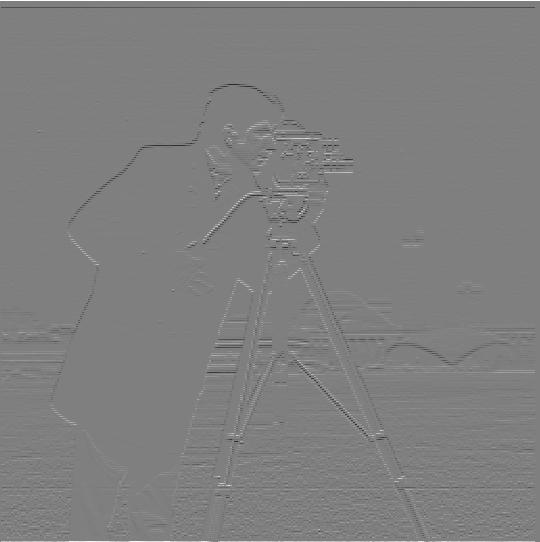
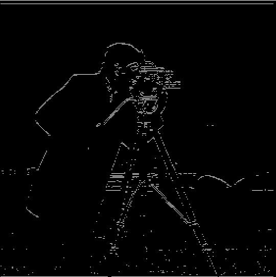
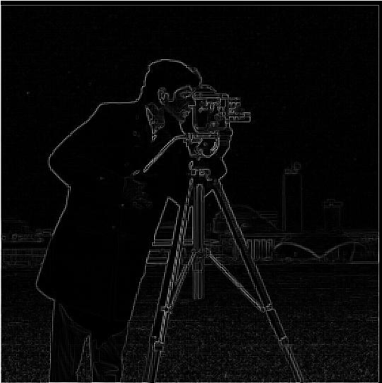
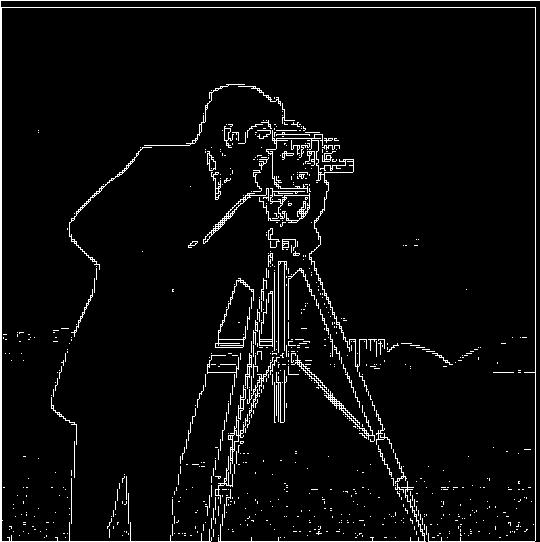
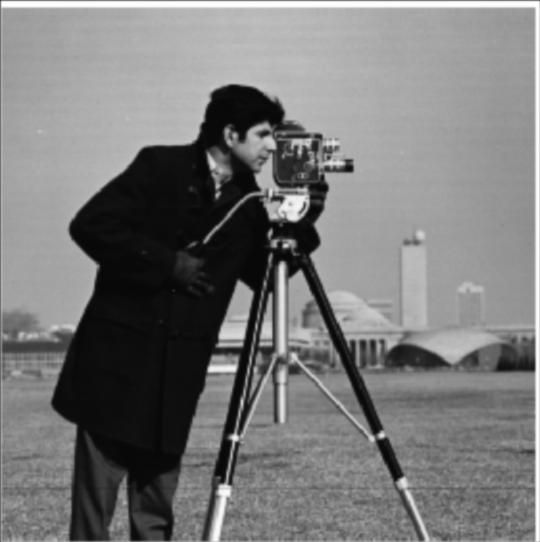
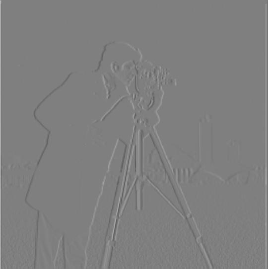
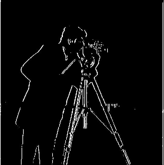
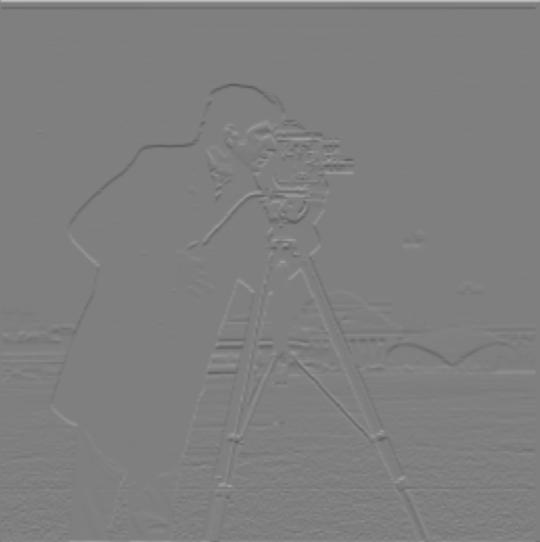
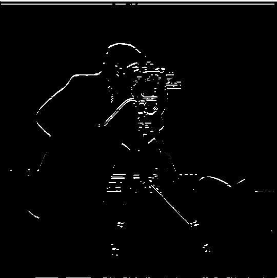
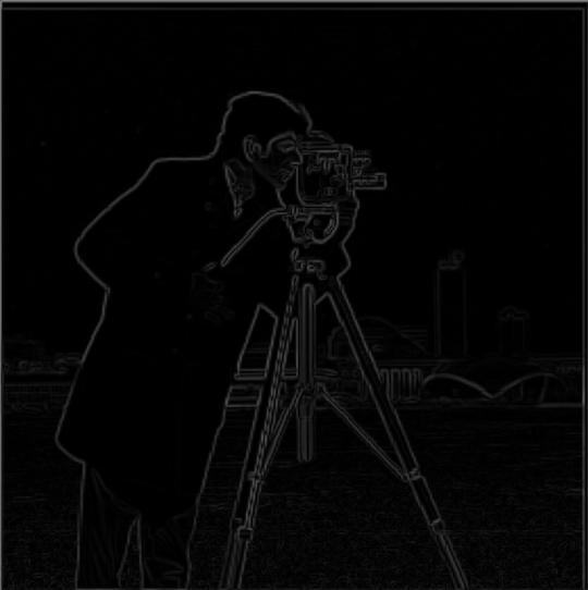
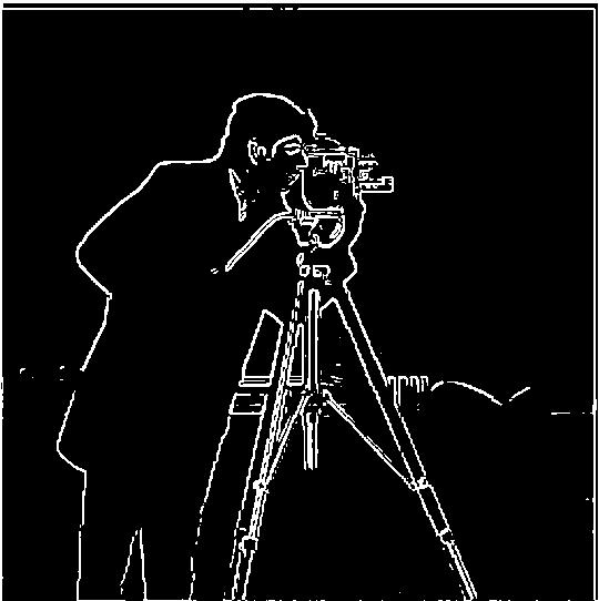
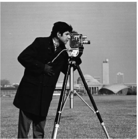
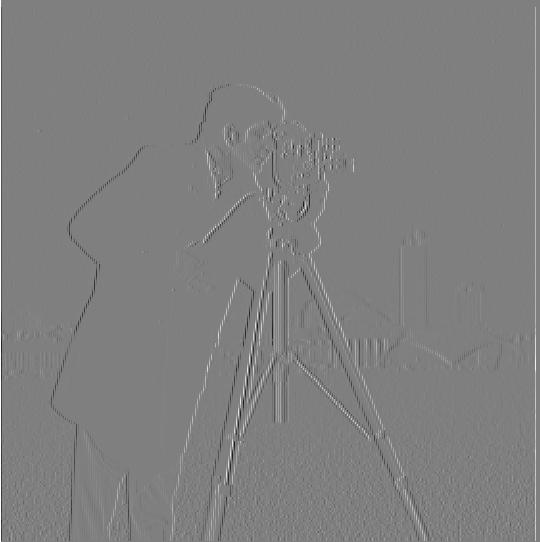
The finite difference operator has the following formulation: Finite Difference matrix

We apply these filters to the cameraman image shown below. Note that we rescale the -1 to 1 possible difference range into 0 to 1 in order to display negative derivative values properly. To calculate the gradient magnitude, we element-wise take the square root of the sum of the square of pixel values for dx and dy. To compute the binary edge image, we use a threshold of 0.2 on the gradient magnitude/absolute value of partial difference.

	Cameraman Original Image
	Raw	Binarized
Dx
Dy
Magnitude

Part 1.2: Derivative of Gaussian

We note that this difference operation is quite noisy. While we tried our best to pick the correct binary threshold, we see quite a bit of noise in the edge detection, especially in the bottom of the image. To fix this, we can apply some smoothing of the image, so that only actual edges lead to a large finite difference. We first apply a Gaussian blur using a filter of sigma 1 and kernel size 10. Then, we apply the same finite difference operations discussed above, except we use a lower threshold of 0.1 since the smoothing reduces the overall magnitude of differences. This creates the following results:

	Cameraman Blurred
	Raw	Binarized
Dx
Dy
Magnitude

When comparing the two sets of images, we see that the finite difference plots have much thicker lines, which makes sense, as the effective averaging of the blur spreads the edge over a larger region. We also see that the binarized image of the edge filter has a lot stronger, clearer lines with less noise. The noise that we saw in the gradient magnitude binary image in the bottom of the image is almost completely gone. For sake of easier comparison, the binary gradient magnitude images are reproduced with and without gaussian filtering.

	Finite Difference	Finite Difference w/ Gaussian Filtering
Binarized Gradient Magnitude

We also change the order of the convolution and first convolve the difference and gaussian blur filters, and then convolve the image with this. Since convolution is commutative, the images are the same apart from floating point error. We note it is important to use full convolution, otherwise convolution is clearly not commutative (even the size changes based on order of operands). Below compares the (identical) Dx and Dy calculated through the two difference ways:

	Finite Difference on Blurred	Derivative of Gaussian Filter
Dx
Dy

We see that they are the same, as expected.

Part 2: Fun With Frequencies

Part 2.1: Image Sharpening

Approach

To perform sharpening, we want to add more high frequencies. To keep the high frequencies, we want so subtract the blurred image from the original image, and add a multiple of this difference to the original image. We can express this as one convolution. Here is the derivation:
Sharpen Filter Derivation

Thus, we calculate the sharpen filter as the sum of a delta and alpha times delta minus our Gaussian. To make sure delta is well defined, we use an odd kernel size, which is the odd number closest to 6 times the provided sigma value. We also adjust the size of our images accordingly to be around 1000 in the largest direction, otherwise the process is a bit slow. It is very important to clip the pixel values to avoid weird overflow and underflow errors.

Results

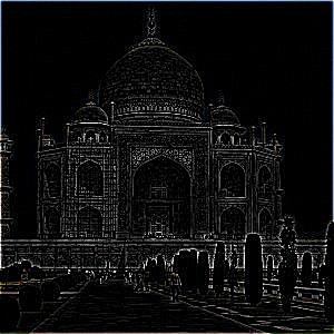
We first look at the results of the image Taj Mahal. This image was sharpened with alpha = 4 and sigma = 1. The sharpened details is shown below, and then the image before and after sharpening, along with a few other sharpened images.

	Taj Mahal Sharpening Details
	Original Image	After Sharpening
Taj Mahal [alpha = 4, sigma = 1]
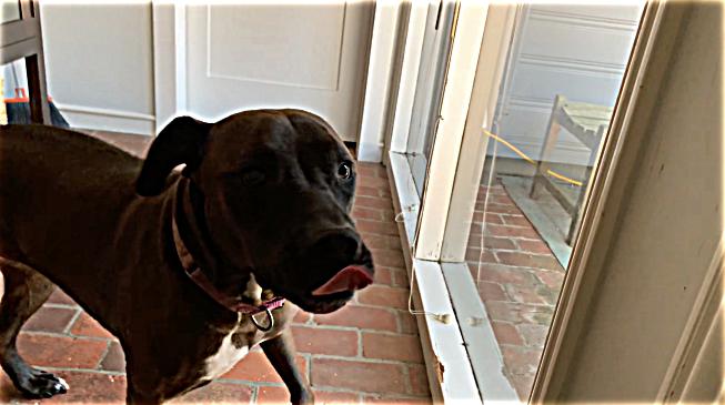
Bear (My Dog) [alpha = 2, sigma = 3]
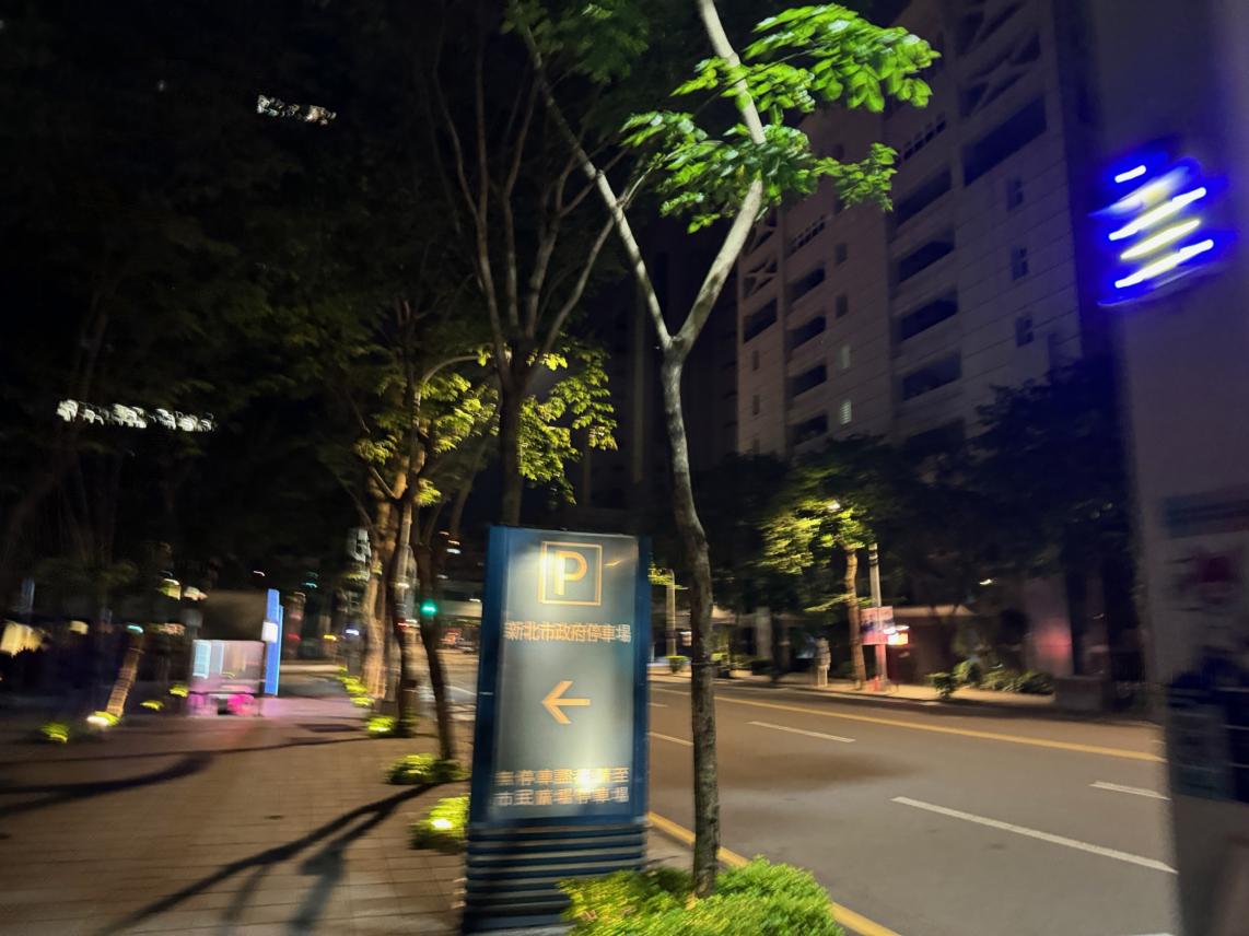
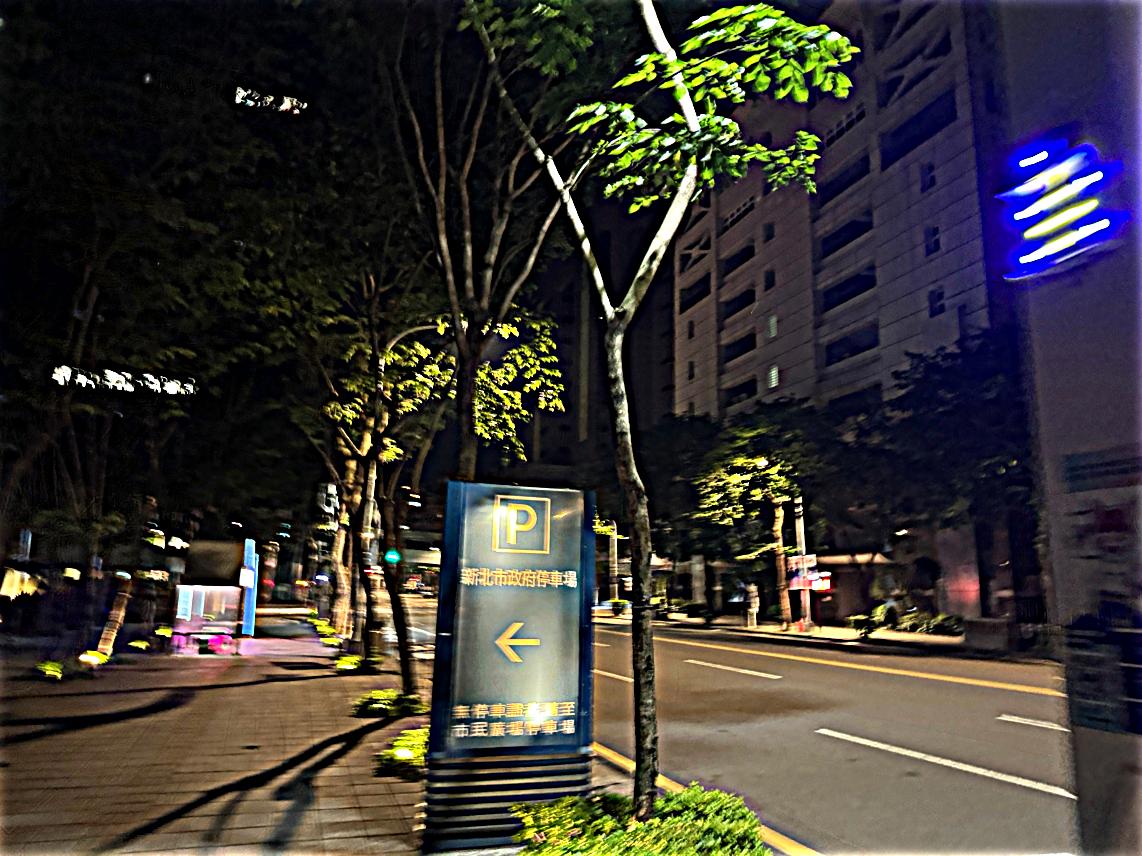
Banqiao District, New Taipei (板桥区，新北市) [alpha = 2, sigma = 5]

We see that the details isolated is the high frequency aspects of the image, which includes all of the edges. Thus, it makes sense that when we add the high frequency components to the original image, the edges become more visible, leading to the perception of a sharper image.

We see that the picture of Bear also seems a bit sharper, as well as the street picture in Banqiao, though the blur is at a low enough frequency that it is difficult to fix this issue by adding high frequencies that are missing in large parts of the image. The bricks in the picture of Bear are more clearly separated, as are the leaves in the Banqiao picture.

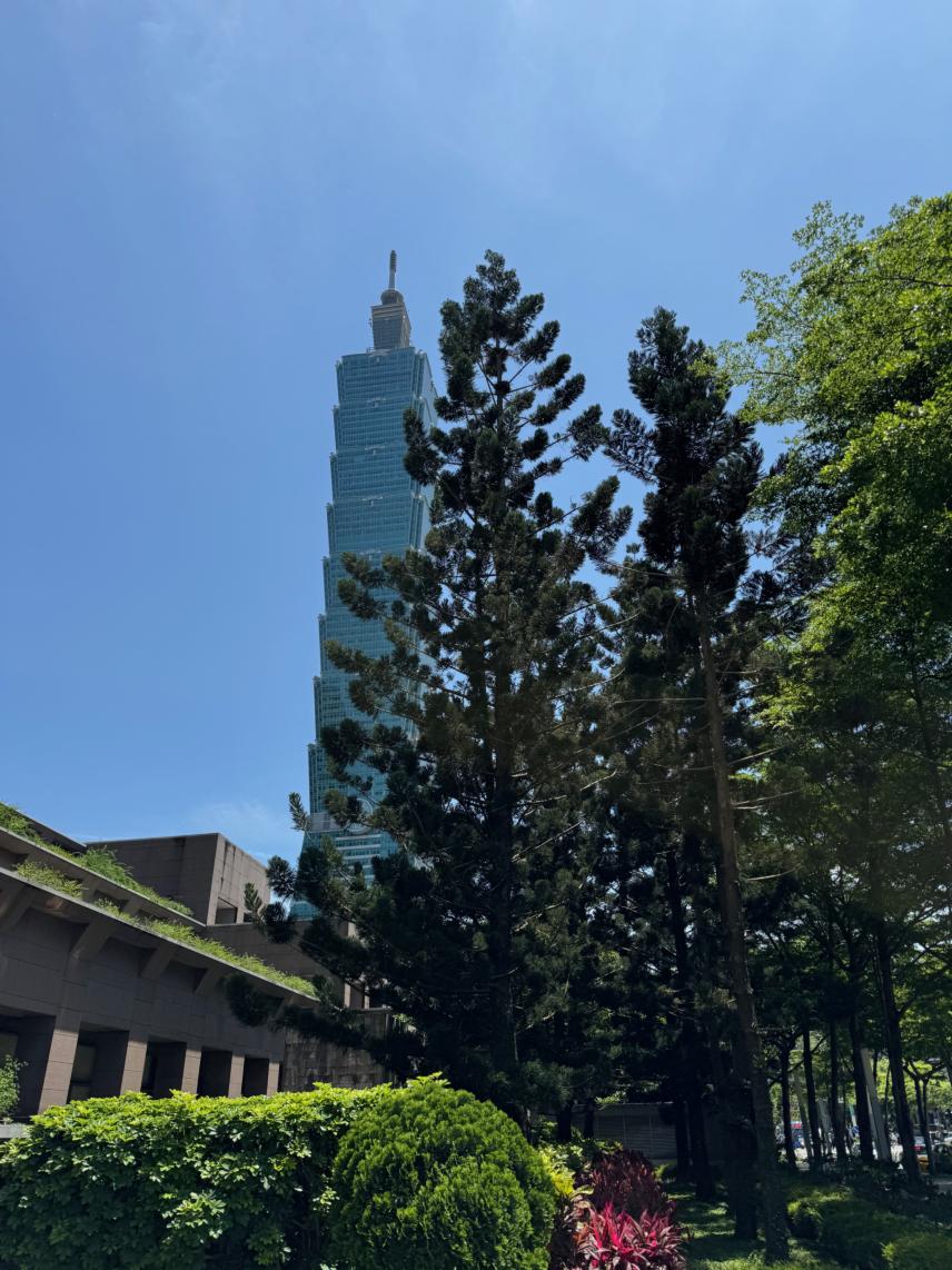
We can also take an image that is sharp, blur it, and then resharpen it. Below is the original image, blurred image, and sharpened image:

	Taipei 101 Original Sharp Image
	Original (Blurred) Image	After Sharpening
Taipei 101 [alpha = 3, sigma = 3]

We see that as expected, once the high frequencies are removed by blurring, adding more of the existing high frequencies cannot reproduce the original image. The edges have more contrast than the blurred image, so they look a bit more clear, however because of the blurring they are thicker and still not sharp. I think this shows that sharpening can only help with very slight/minor blurring that does not erase most of the high frequencies.

All of the additional photos in this section were taken by me.

Part 2.2: Hybrid Images

Approach

We use the same low pass procedure from above, and the high pass portion of the sharpening procedure (delta - g). We apply low pass filter to one aligned image, high pass filter to the other, and then sum the results. We find that adding works a little bit better, because the image tends to get darker when doing averaging since the high frequency part is zero in many areas of the image. To tune the sigma values for each filter, we try to increase sigma for the high pass until we can see the high frequency image. We tune the sigmas through a fair amount of trial and error. If the high pass image isn't visible, increase sigma. If the low pass isn't visible, reduce it's sigma value. After some amount of trial and error, we generally found suitable sigma values. The kernel size is the closest odd number to 6 times sigma. This method for constructing hybrid images leads to the perception of two images since when the viewer is close, they see the high frequency components and thus the high frequency image, but when they move far away they can only percieve the low frequency filtered image.

Results

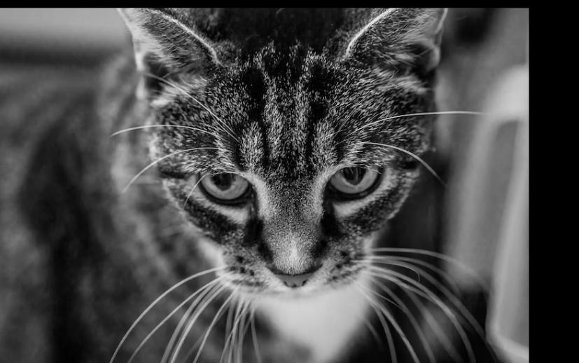
Derek + Nutmeg

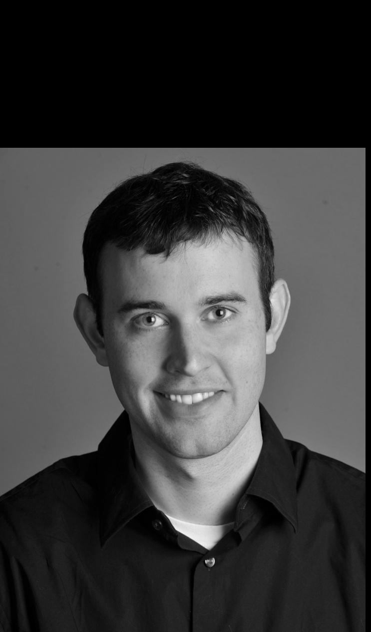
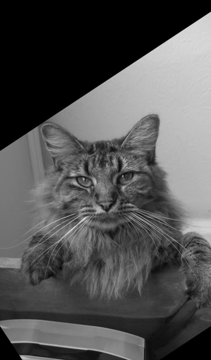
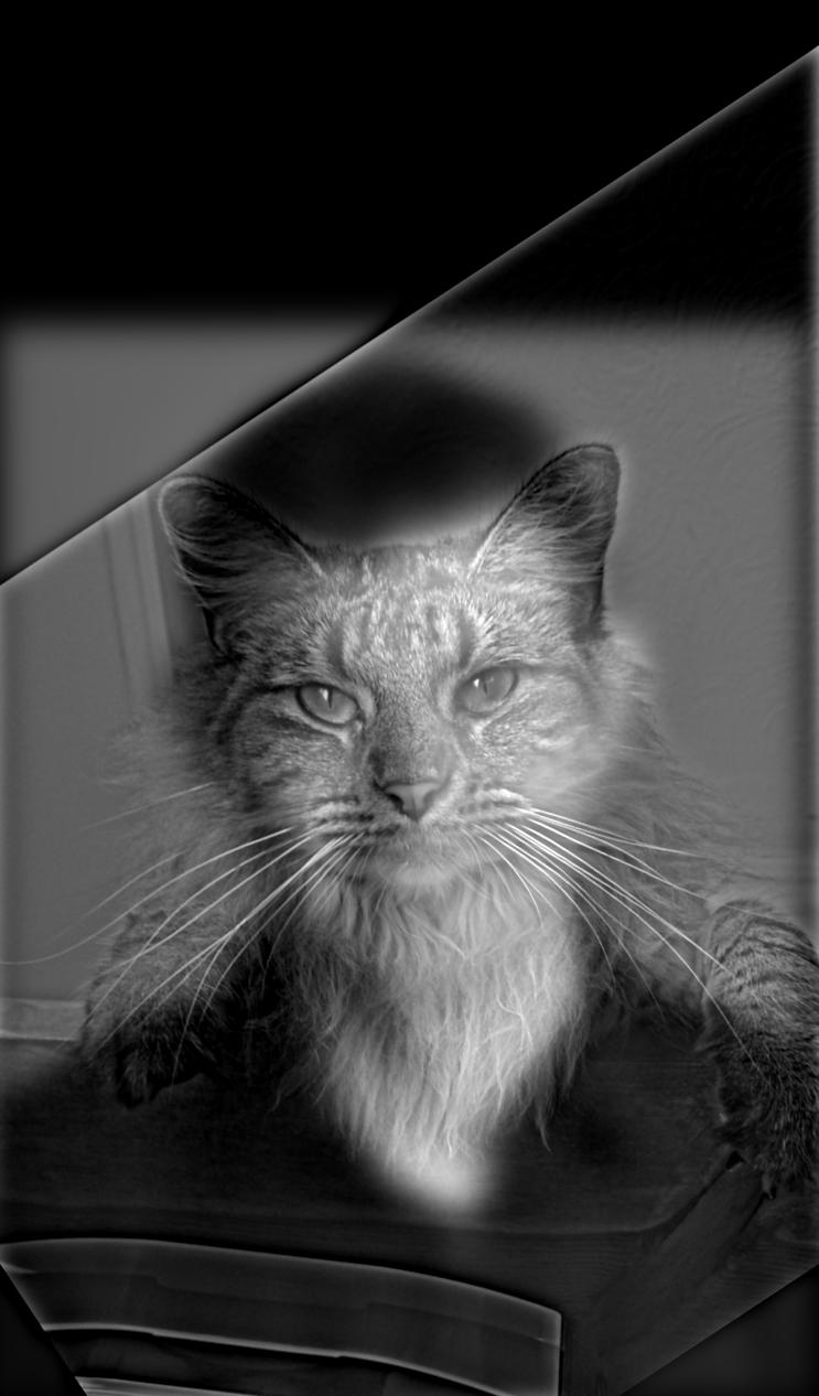
First, we show the results for the picture of Derek and nutmeg, where the low pass sigma was 15 and high pass sigma was 8.

Derek (Low)	Nutmeg (High)

Derek + Nutmeg Hybrid Image

We see that this image combination works quite well, since the proportions of the features of the cat and Derek line up reasonably well, the lighting is similar, and both pictures are completely head on so a translation/rotation based alignment is sufficient.

The Duality of Happiness and Sadness (Favorite)

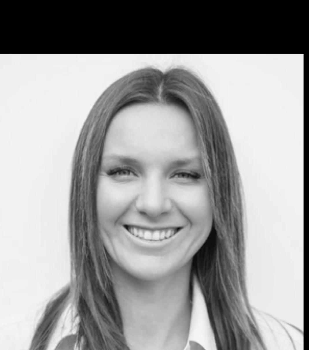
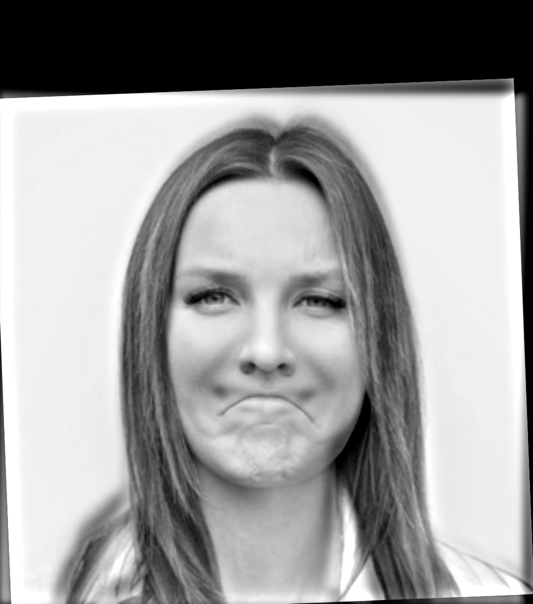
We also use some stock images found online taken by Creative Cat Studio of a woman with various facial expressions. I thought this would work well since the image is otherwise almost completely the same. The low pass sigma is 8 and the high pass sigma is 16.

Happy (Low)	Sad (High)

Happiness + Sadness Hybrid Image

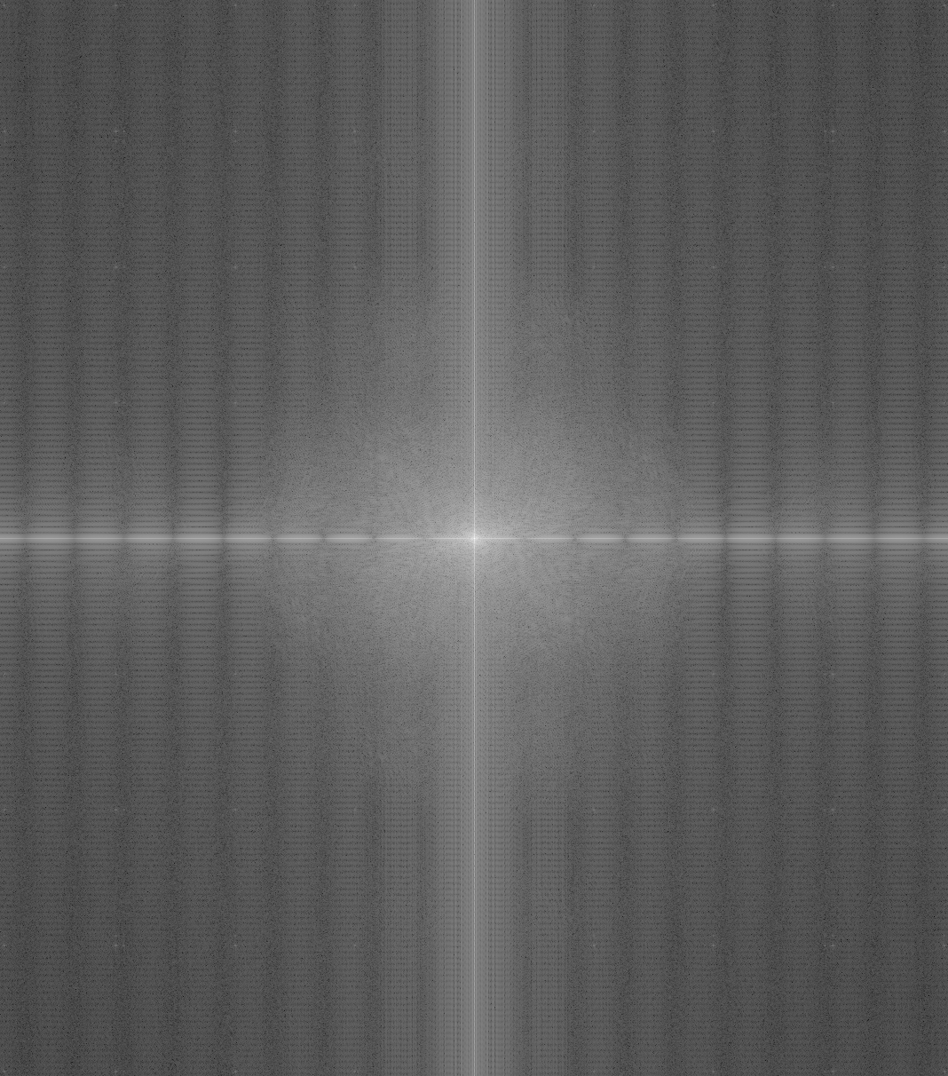
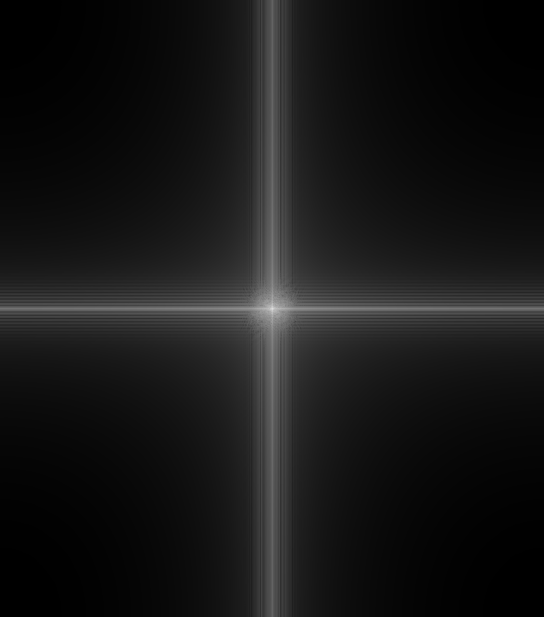
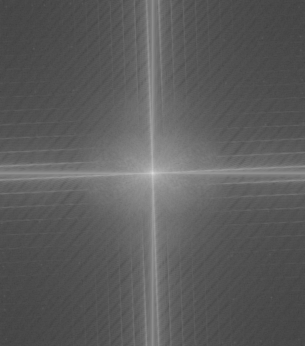
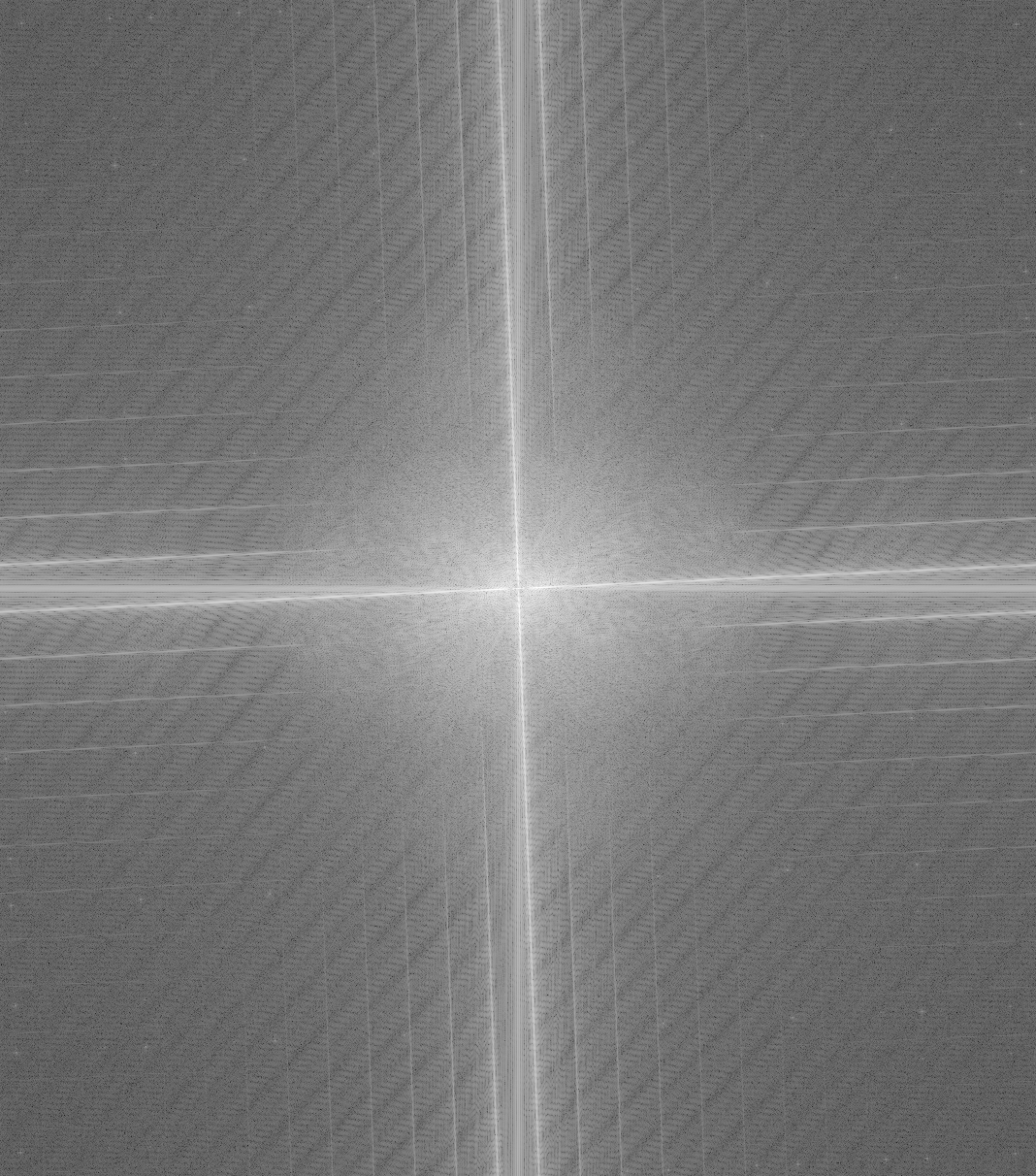
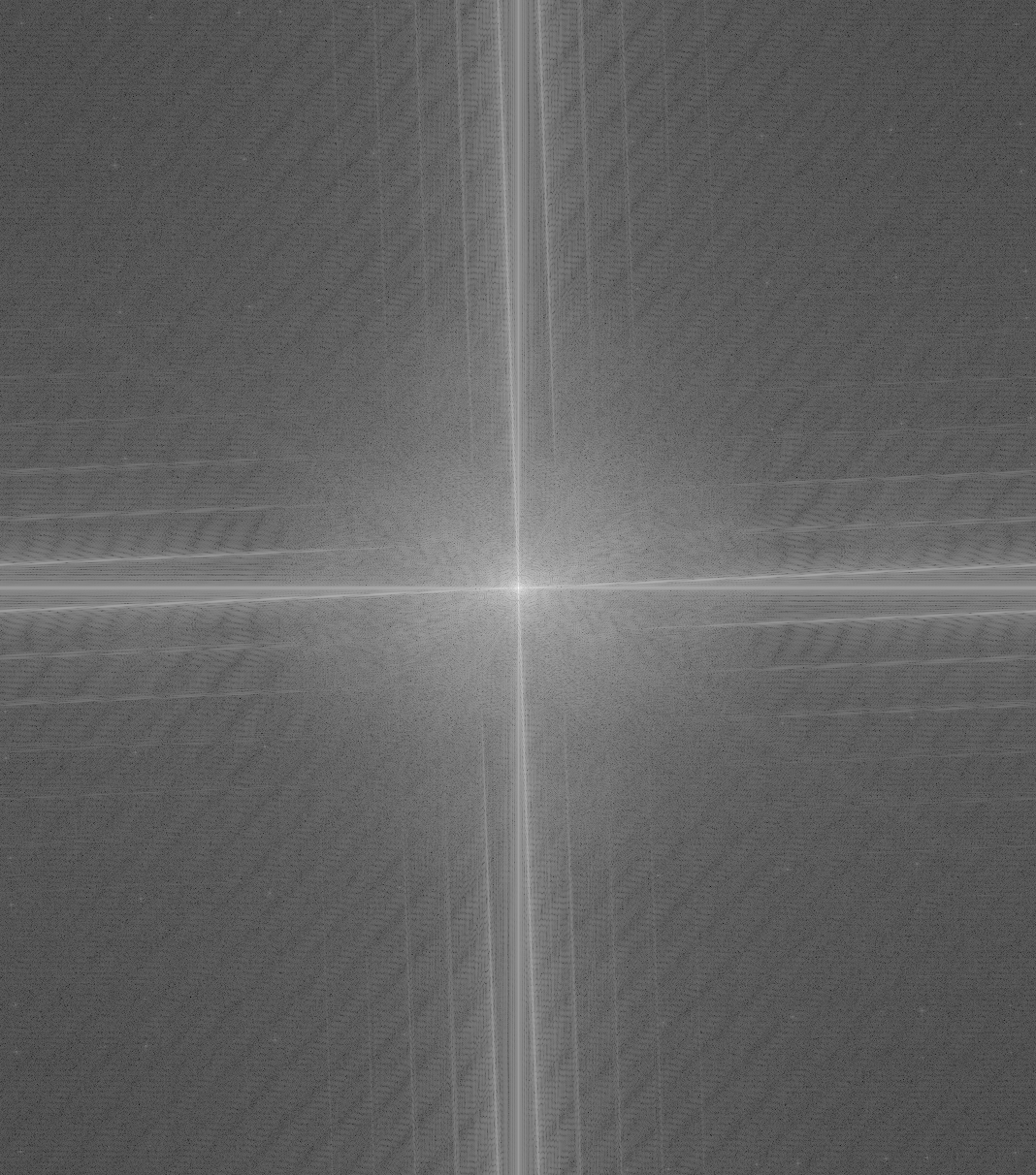
We can plot the log magnitude of the fourier transform of both images before and after filtering, as well as the resulting image to get intuition as to what is happening.

	Original Image FFT	FFT After Filtering
Low Frequency (Happy)
High Frequency (Sad)
	Hybrid Image Plot

We see that for the happy image, most high frequencies are heavily attenuated, as desired, since the color becomes quite dark if the absolute value of fx or fy is high. Similarly, for the high frequency part, after filtering, we see that the bright region expands to cover higher frequencies. This makes sense, since the high pass filter reduces magnitude of low frequencies, but does not add high frequencies. This means that the area that originally was not the whitest color is now the whitest color (it is now the maximum intensity since lower frequencies that used to be close to maximum magnitude have been attenuated). We see that the hybrid image mixes both of these.

Pug and Cat

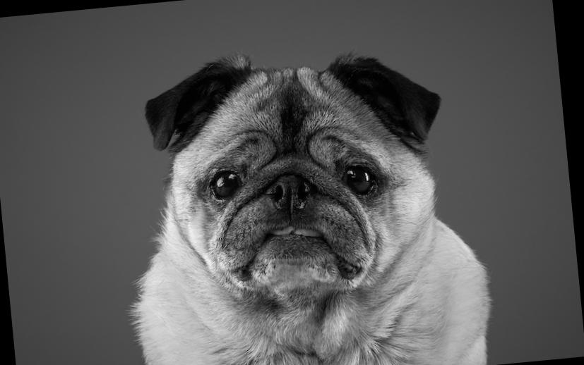
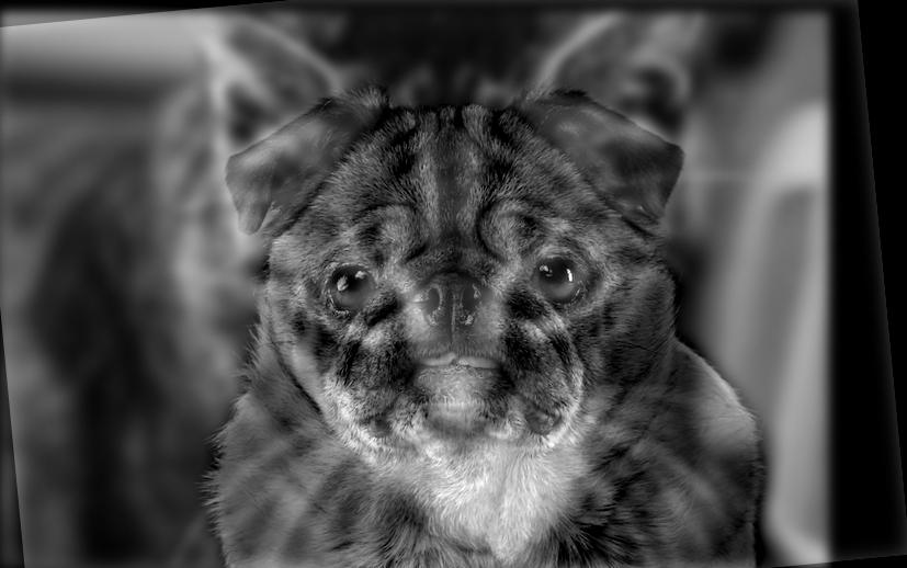
I used some Adobe stock images of a pug and cat to create the following hybrid image. The sigma for low filter is 5, sigma for high filter is 8.

Cat (Low)	Pug (High)

Cat and Pug Hybrid Image

This seems to work reasonably well, but not quite as clear as the first, since the images are quite different which is a bit distracting.

Flower (Failure)

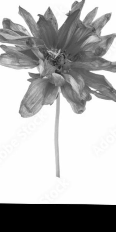
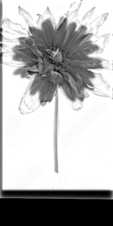
I also tried to do a flower, where the low frequency was a healthy flower and the high frequency was a dying flower. Unfortunately, since the healthy flower has a white background around it, you don't really every stop seeing the dying flower. There is also some sizing issues. This shows that you need similar sized images with similar lighting and a background for high frequency to disappear into. Low pass sigma is 3, high pass is 8.

Blooming Flower (Low)	Dying Flower (High)

Blooming and Dying Flower Hybrid Image

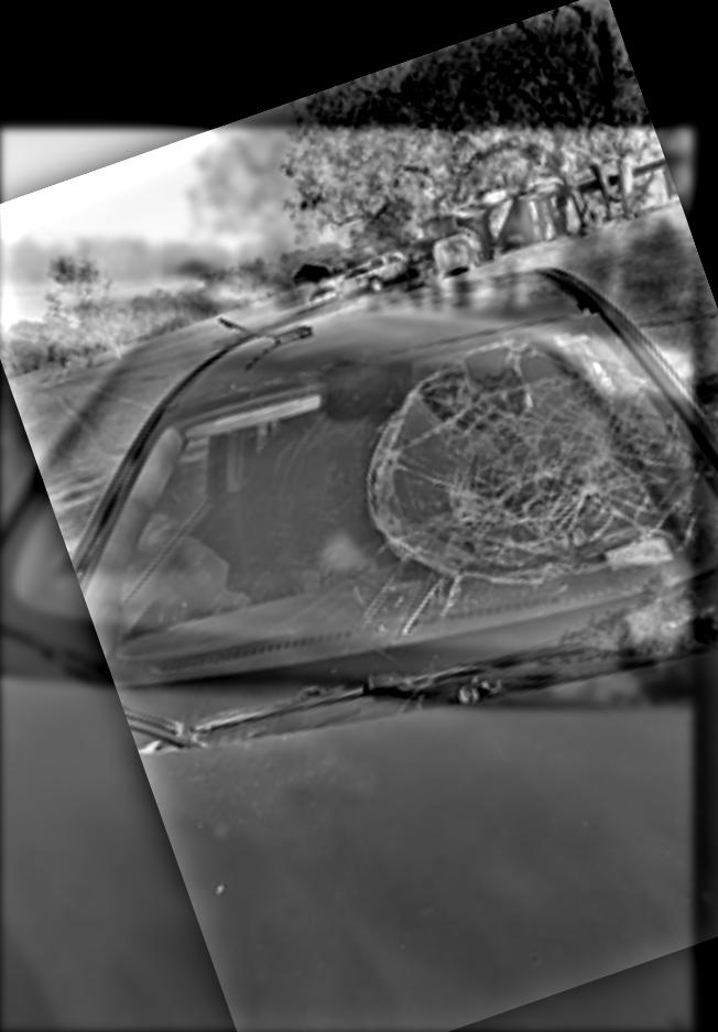
Car Windshield (Failure)

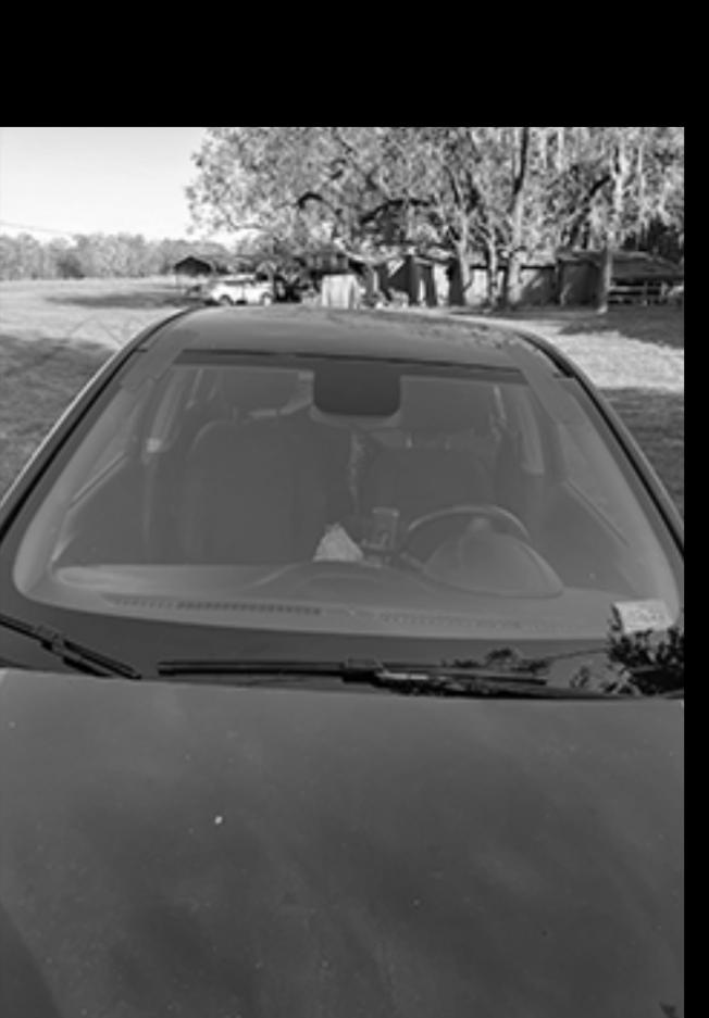
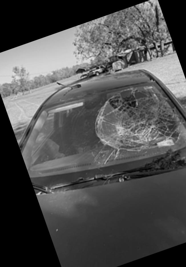
I also tried to do a car windshield, where the low frequency was an intact windshield and a high frequency was a broken windshield. Again, these pictures were very difficult to align since the angle was not quite the same. Also, its still hard for the cracks to disappear with distance. We used low pass filter sigma of 4 and high pass sigma of 16.

Intact Windshield (Low)	Broken Windshield (High)

Intact and Broken Windshield Hybrid Image

Part 2.3: Laplacian and Gaussian Stacks

Approach

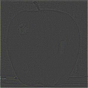
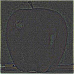
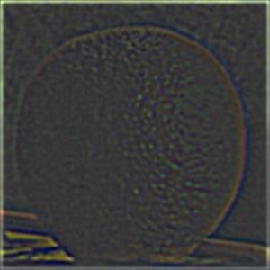
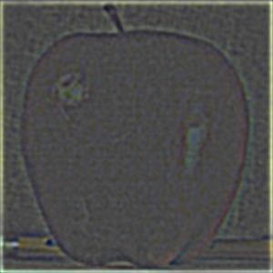
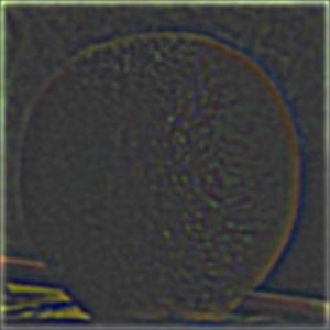
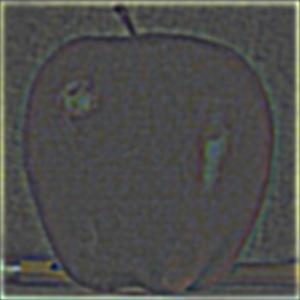
To compute the Gaussian stack, we repeatedly apply a Gaussian filter with a specified sigma to create a Gaussian stack of a specified level. We use one with 8 levels. We then compute the Lagrangian stack as the difference between level i + 1 and level i for i in the range of [0, 6]. For the last level of the Laplacian stack, we use the last level of the Gaussian stack. That way, they have the same number of levels and the sum of the Laplacian stack is the original image. This means the Laplacian stack just partitions the frequencies of the original image. For these visualizations of the apple and orange, we use a sigma of 1, and kernel size is calculated same as above. For ease of visualization, we normalize each image so the lowest value is 0, and highest value is 1.

Results

Below we show the Laplacian stack at levels 0, 2, 4, 6 for the apple and orange.

	Orange	Apple
Level 0
Level 2
Level 4
Level 6

We note that at each later level, the features are coarser, which makes sense since they are lower frequency. Ours don't get quite as course as the original paper since our sigma value is likely higher, however in practice for performing merging this seems to be a good parameter, and also has faster performance due to the small filter size.

Part 2.4: Multiresolution Blending

Approach

We first take the stacks from above (all with a sigma of 1 and 8 levels). We also create a blending mask and create a Gaussian stack for this mask with the same number of levels as the image stacks. Then, we multiply the first image Laplacian times the mask Gaussian stack element-wise for the first image, and the Laplacian stack for the second image times one minus the Gaussian stack. Then, we add these stacks and sum over all levels. The only parameter that I changed between images is the amount of blurring at each level for the Gaussian stack for the mask.

Results

Dog With Human Smile (Favorite)

We first show the result of fusing a dog image with a human mouth image. Both images are from Adobe Stock. To create the irregular mask and align the images, I used Photoshop and then exported layers separately. We used a sigma of 5 for the mask Gaussian stack blur. Below are the individual aligned images:

Dog	Smiling Person	Mask

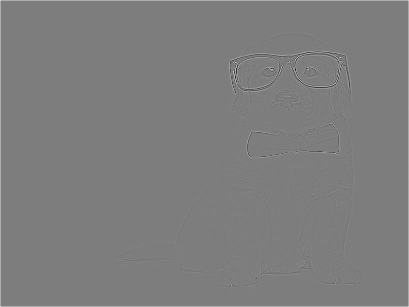
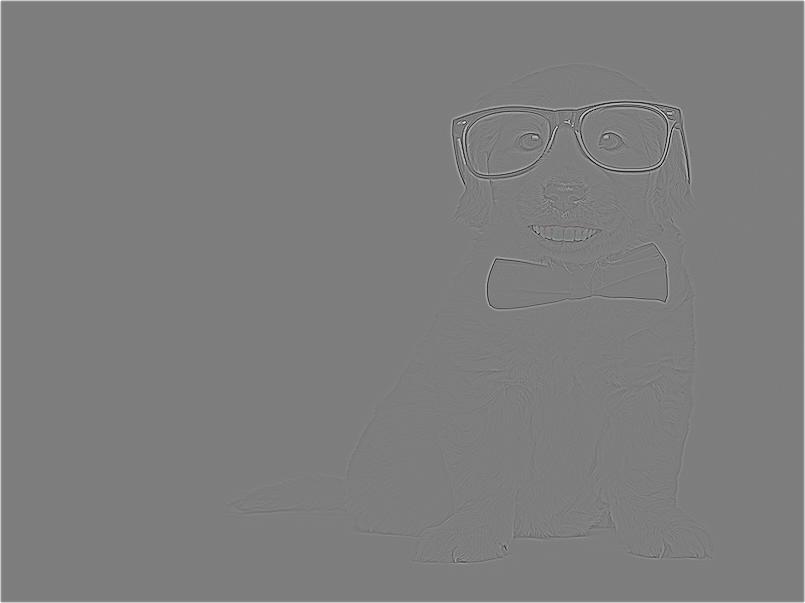
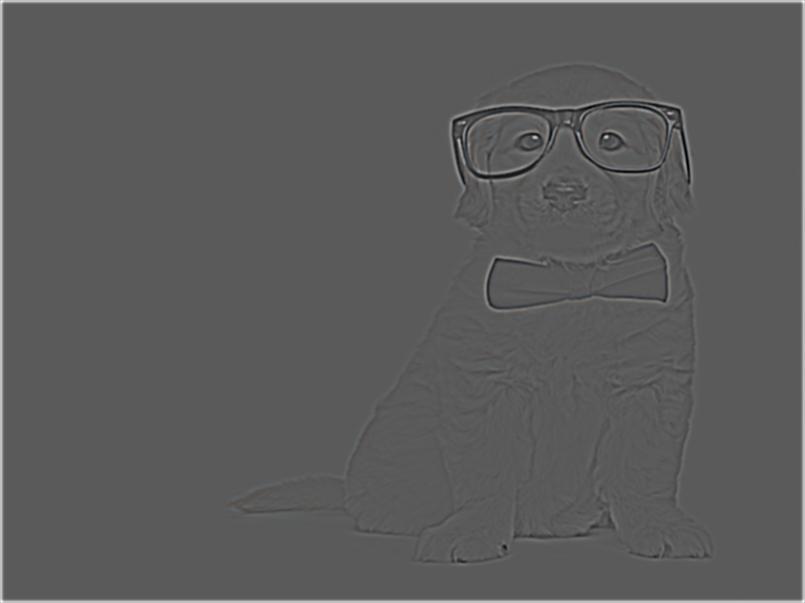
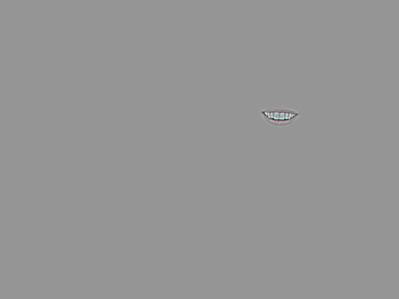
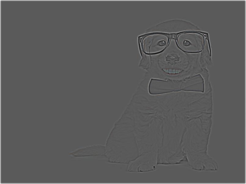
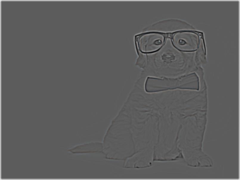
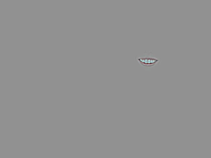
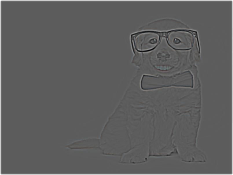
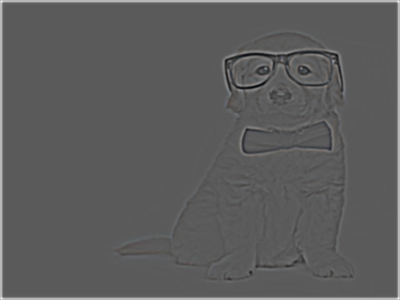
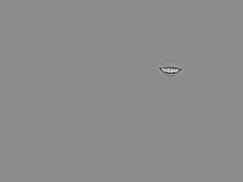
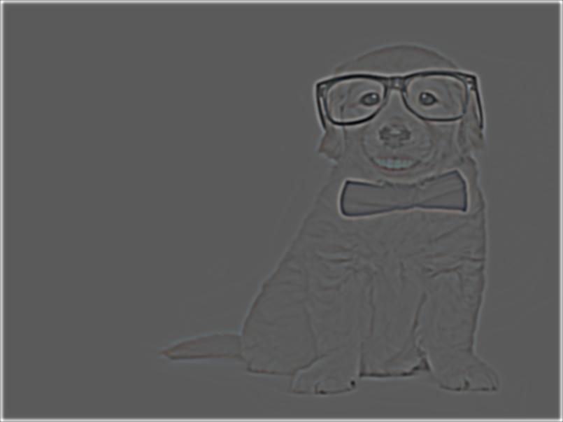
Now, below, we show the intermediate Laplacian levels and the blended combination of each level. Each level is normalized, but it can still be a bit hard to see because most the image has nothing and is thus the same color.

	Dog	Smiling Person	Blended At Level
Level 0
Level 2
Level 4
Level 6

Now, we show the final image, and observe that the multi-resolution blending leads to a much smoother, better result than the Photoshop mockup that does not do any blending:

Photoshop (No Blending)	Multiresolution Blending

Samsung Galaxy S24 Ultra + iPhone 15 Pro Max

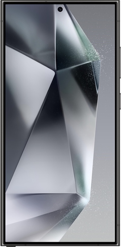
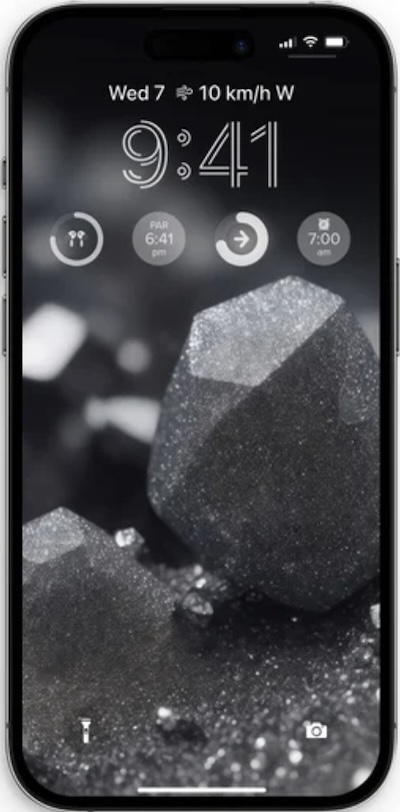
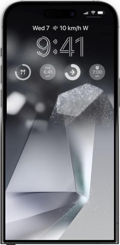
I also made a multiresolution blend of a Samsung Galaxy S24 Ultra and iPhone 15 Pro Max. Images were sourced from here and here used a sigma of 11 for my mask Gaussian stack, and a horizontal 50-50 mask. The images are shown below, as well as the final result:

S24 Ultra	iPhone 15 Pro Max

S24 Ultra and iPhone 15 Pro Max Fused Image

Orapple

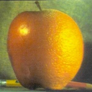
Finally, we reproduce the orange-apple merge from the original 1983 paper by Burt and Adelson. We use a vertical 50-50 split mask, and the same sigma value of 11. Below are the original images and fused image:

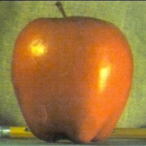
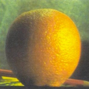
Apple	Orange

Apple and Orange Fused Image